## Uncomment the following lines to set up the python environment
## Probably not needed depending on where you are running this notebook

#!pip install torch
#!pip install nilearn
#!pip install nibabel
#!pip install pandas
#!pip install sklearn
#!pip install matplotlib
#!pip install numpy
#!pip install torch torchvision
!git clone https://gitlab.inria.fr/epione_ML/mcvae.git
import sys
import os
sys.path.append(os.getcwd() + '/mcvae/src/')
import mcvae
print('Mcvae version:' + mcvae.__version__)
fatal: destination path 'mcvae' already exists and is not an empty directory.
Mcvae version:2.0.0
import numpy as np
import matplotlib.pyplot as plt
%matplotlib inline
from sklearn.cross_decomposition import PLSCanonical, CCA
Random data generation
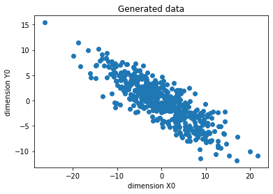
Our journey in the analysis of heterogeneous data starts with the generation of synthetic data. We first need to generate multivarite correlated random variables X and Y. To do so, we rely on the generative model we have seen during lesson:
# #############################################################################

# N subjects
n = 500
# here we define 2 Gaussian latents variables z = (l_1, l_2)
np.random.seed(42)
l1 = np.random.normal(size=n)
l2 = np.random.normal(size=n)

latents = np.array([l1, l2]).T

# We define two random transformations from the latent space to the space of X and Y respectively
transform_x = np.random.randint(-8,8, size = 10).reshape([2,5])
transform_y = np.random.randint(-8,8, size = 10).reshape([2,5])

# We compute data X = z w_x, and Y = z w_y
X = latents.dot(transform_x)
Y = latents.dot(transform_y)

# We add some random Gaussian noise
X = X + 2*np.random.normal(size = n*5).reshape((n, 5))
Y = Y + 2*np.random.normal(size = n*5).reshape((n, 5))


print('The latent space has dimension ' + str(latents.shape))
print('The transformation for X has dimension ' + str(transform_x.shape))
print('The transformation for Y has dimension ' + str(transform_y.shape))

print('X has dimension ' + str(X.shape))
print('Y has dimension ' + str(Y.shape))
The latent space has dimension (500, 2)
The transformation for X has dimension (2, 5)
The transformation for Y has dimension (2, 5)
X has dimension (500, 5)
Y has dimension (500, 5)
dimension_to_plot = 0

plt.scatter(X[:,1], Y[:,2])
plt.xlabel('dimension X' + str(dimension_to_plot))
plt.ylabel('dimension Y' + str(dimension_to_plot))
plt.title('Generated data')
plt.plot()
[]
PLS and scikit-learn: basic use
Our newly generated data can be already used to test the PLS and CCA provided by standard machie learning packages, such as scikit-learn.
##########################################################
# We first split the data in trainig and validation sets

# The training set is composed by a random sample of dimension N/2
train_idx = np.random.choice(range(X.shape[0]), size = int(X.shape[0]/2), replace = False)
X_train = X[train_idx, :]

# The testing set is composed by the remaining subjects
test_idx = np.where(np.in1d(range(X.shape[0]), train_idx, assume_unique =True, invert = True))[0]
X_test = X[test_idx, :]

# We reuse the same indices to split the data Y
Y_train = Y[train_idx, :]
Y_test = Y[test_idx, :]
#######################################
# We fit PLS as provided by scikit-learn

#Defining PLS object
plsca = PLSCanonical(n_components=2)

#Fitting on train data
plsca.fit(X_train, Y_train)

#We project the training data in the latent dimension
X_train_r, Y_train_r = plsca.transform(X_train, Y_train)
#We project the testing data in the latent dimension
X_test_r, Y_test_r = plsca.transform(X_test, Y_test)
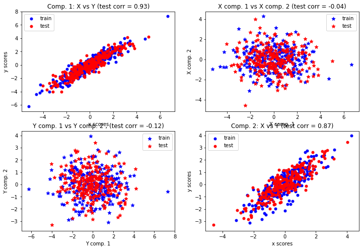
We note that the projections in the latent space retrieved by PLS are indeed correlated. The different dimensions of the projections are however uncorrelated.
# Scatter plot of scores
# ~~~~~~~~~~~~~~~~~~~~~~
# 1) On diagonal plot X vs Y scores on each components
plt.figure(figsize=(12, 8))
plt.subplot(221)
plt.scatter(X_train_r[:, 0], Y_train_r[:, 0], label="train",
            marker="o", c="b", s=25)
plt.scatter(X_test_r[:, 0], Y_test_r[:, 0], label="test",
            marker="o", c="r", s=25)
plt.xlabel("x scores")
plt.ylabel("y scores")
plt.title('Comp. 1: X vs Y (test corr = %.2f)' %
          np.corrcoef(X_test_r[:, 0], Y_test_r[:, 0])[0, 1])

plt.legend(loc="best")

plt.subplot(224)
plt.scatter(X_train_r[:, 1], Y_train_r[:, 1], label="train",
            marker="o", c="b", s=25)
plt.scatter(X_test_r[:, 1], Y_test_r[:, 1], label="test",
            marker="o", c="r", s=25)
plt.xlabel("x scores")
plt.ylabel("y scores")
plt.title('Comp. 2: X vs Y (test corr = %.2f)' %
          np.corrcoef(X_test_r[:, 1], Y_test_r[:, 1])[0, 1])

plt.legend(loc="best")

# 2) Off diagonal plot components 1 vs 2 for X and Y
plt.subplot(222)
plt.scatter(X_train_r[:, 0], X_train_r[:, 1], label="train",
            marker="*", c="b", s=50)
plt.scatter(X_test_r[:, 0], X_test_r[:, 1], label="test",
            marker="*", c="r", s=50)
plt.xlabel("X comp. 1")
plt.ylabel("X comp. 2")
plt.title('X comp. 1 vs X comp. 2 (test corr = %.2f)'
          % np.corrcoef(X_test_r[:, 0], X_test_r[:, 1])[0, 1])
plt.legend(loc="best")


plt.subplot(223)
plt.scatter(Y_train_r[:, 0], Y_train_r[:, 1], label="train",
            marker="*", c="b", s=50)
plt.scatter(Y_test_r[:, 0], Y_test_r[:, 1], label="test",
            marker="*", c="r", s=50)
plt.xlabel("Y comp. 1")
plt.ylabel("Y comp. 2")
plt.title('Y comp. 1 vs Y comp. 2 , (test corr = %.2f)'
          % np.corrcoef(Y_test_r[:, 0], Y_test_r[:, 1])[0, 1])
plt.legend(loc="best")

plt.show()
#We can check the estimated projections
print('X projections: \n' + str(plsca.x_weights_))

print('Y projections: \n' + str(plsca.y_weights_))
X projections:
[[ 0.48433579 -0.25654367]
 [-0.51415729  0.28837788]
 [ 0.57083361  0.41523051]
 [-0.1600194   0.72474008]
 [-0.38678665 -0.39161076]]
Y projections:
[[ 0.36148438  0.39913339]
 [-0.39571466  0.70730378]
 [ 0.49905721 -0.35689321]
 [-0.48904463 -0.31141709]
 [-0.4738314  -0.34067659]]
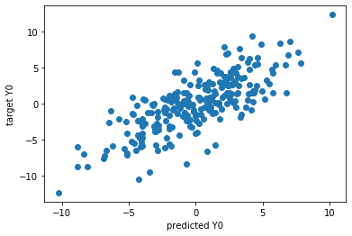
# Prediction for the training data

predicted_Y_train = plsca.predict(X_train)

plt.scatter(predicted_Y_train[:,dimension_to_plot], Y_train[:,dimension_to_plot])
plt.ylabel('target Y' + str(dimension_to_plot))
plt.xlabel('predicted Y' + str(dimension_to_plot))

plt.show()
plsca_4 = PLSCanonical(n_components=4)
plsca_4.fit(X_train, Y_train)

predicted_Y_train = plsca_4.predict(X_train)

print('X projections with 2 components: \n' + str(plsca.x_weights_))

print('Y projections with 2 components: \n' + str(plsca.y_weights_))

print('X projections with 4 components: \n' + str(plsca_4.x_weights_))

print('Y projections with 4 components: \n' + str(plsca_4.y_weights_))
X projections with 2 components:
[[ 0.48433579 -0.25654367]
 [-0.51415729  0.28837788]
 [ 0.57083361  0.41523051]
 [-0.1600194   0.72474008]
 [-0.38678665 -0.39161076]]
Y projections with 2 components:
[[ 0.36148438  0.39913339]
 [-0.39571466  0.70730378]
 [ 0.49905721 -0.35689321]
 [-0.48904463 -0.31141709]
 [-0.4738314  -0.34067659]]
X projections with 4 components:
[[ 0.48433579 -0.25654367 -0.42402831  0.54660349]
 [-0.51415729  0.28837788  0.30201819  0.74306133]
 [ 0.57083361  0.41523051  0.64183921 -0.06465157]
 [-0.1600194   0.72474008 -0.51490022 -0.22931801]
 [-0.38678665 -0.39161076  0.22782708 -0.30383862]]
Y projections with 4 components:
[[ 0.36148438  0.39913339 -0.5105896   0.60783454]
 [-0.39571466  0.70730378  0.48505202  0.26714451]
 [ 0.49905721 -0.35689321  0.58283628  0.50546537]
 [-0.48904463 -0.31141709  0.17782666  0.30291833]
 [-0.4738314  -0.34067659 -0.36428334  0.46034359]]
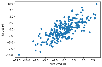
# We can also predict Y from X

predicted_Y_test = plsca.predict(X_test)

plt.scatter(predicted_Y_test[:,dimension_to_plot], Y_test[:,dimension_to_plot])
plt.ylabel('target Y' + str(dimension_to_plot))
plt.xlabel('predicted Y' + str(dimension_to_plot))

plt.show()
Exercise. Generate a synthetic dataset of 200 observations.
Each observation is composed by 3 modalities X1, X2, and X3, of dimensions respectively of 4, 7, and 9.
Chose the appropriate latent variable representation for the generative model.
These modalities are corrupted with Gaussian noise, with different noise variance for each modality.
Fit a PLS model to predict X3 from X1.
Into the guts of latent variable models
After playing with the builti-in implementation of PLS in scikit-learn, we are going to implement our own version based on the NIPALS method.
NIPALS for PLS
# Nipals method for PLS

n_components = 3


# Defining empty arrays where to store results

# Reconstruction from latent space to data
loading_x = np.ndarray([X.shape[1],n_components])
loading_y = np.ndarray([Y.shape[1],n_components])

# Projections into the latent space
weight_x = np.ndarray([X.shape[1],n_components])
weight_y = np.ndarray([Y.shape[1],n_components])

# Latent variables
scores_x = np.ndarray([X.shape[0],n_components])
scores_y = np.ndarray([Y.shape[0],n_components])


# Initialization of data matrices
current_X = X
current_Y = Y

for i in range(n_components):
    # Initialization of current latent variables as a data column
    t_x = current_X[:,0]

    # NIPALS iterations
    for _ in range(100):
        # estimating Y weights given data Y and latent variables from X
        w_y = current_Y.transpose().dot(t_x)/(t_x.transpose().dot(t_x))
        # normalizing Y weights
        w_y = w_y/np.sqrt(np.sum(w_y**2))

        # estimating latent variables from Y given data Y and Y weights
        t_y = current_Y.dot(w_y)
        # estimating X weights given data X and latent variables from Y
        w_x = current_X.transpose().dot(t_y)/(t_y.transpose().dot(t_y))
        # normalizing X weights
        w_x = w_x/np.sqrt(np.sum(w_x**2))

        # estimating latent variables from X given data X and X weights
        t_x = current_X.dot(w_x)

    # Weights are such that X * weights = t
    weight_x[:,i] = w_x
    weight_y[:,i] = w_y

    # Latent variables
    scores_x[:,i] = t_x
    scores_x[:,i] = t_y

    # Loadings obtained by regressing X on t (X = t * loadings)

    loading_x[:,i] = np.dot(current_X.T, t_x)/t_x.transpose().dot(t_x)
    loading_y[:,i] = np.dot(current_Y.T, t_y)/t_y.transpose().dot(t_y)

    # Deflation = current_data - current_reconstruction

    current_X = current_X - t_x.reshape(len(t_x),1).dot(w_x.reshape(1,len(w_x)))
    current_Y = current_Y - t_y.reshape(len(t_y),1).dot(w_y.reshape(1,len(w_y)))
print('The estimated projections for X are: \n' + str(weight_x))

print('\n The estimated projections for Y are: \n' + str(weight_y))
The estimated projections for X are:
[[ 0.36753226  0.32695545  0.31901594]
 [-0.54017132 -0.51142438 -0.13635813]
 [ 0.73596167 -0.54668695 -0.38095079]
 [-0.07131382 -0.54068145  0.43213359]
 [-0.16251074  0.20085364 -0.74011644]]

 The estimated projections for Y are:
[[ 0.22469208 -0.22321827  0.22848154]
 [-0.42360052 -0.82303817 -0.17028297]
 [ 0.34143196  0.23277327 -0.37414229]
 [-0.53070486  0.30658588 -0.6691619 ]
 [-0.60979721  0.35299218  0.57536058]]
plt.figure(figsize=(12, 12))
plt.subplot(3,2,1)
plt.scatter(scores_x[:,0], latents[:,0])
plt.xlabel('PLS 0')
plt.ylabel('ground truth 0')
plt.subplot(3,2,2)
plt.scatter(scores_x[:,0], latents[:,1])
plt.xlabel('PLS 0')
plt.ylabel('ground truth 1')
plt.subplot(3,2,3)
plt.scatter(scores_x[:,1], latents[:,0])
plt.xlabel('PLS 1')
plt.ylabel('ground truth 0')
plt.subplot(3,2,4)
plt.scatter(scores_x[:,1], latents[:,1])
plt.xlabel('PLS 1')
plt.ylabel('ground truth 1')
plt.subplot(3,2,5)
plt.scatter(scores_x[:,2], latents[:,0])
plt.xlabel('PLS 2')
plt.ylabel('ground truth 0')
plt.subplot(3,2,6)
plt.scatter(scores_x[:,2], latents[:,1])
plt.xlabel('PLS 2')
plt.ylabel('ground truth 1')
plt.show()
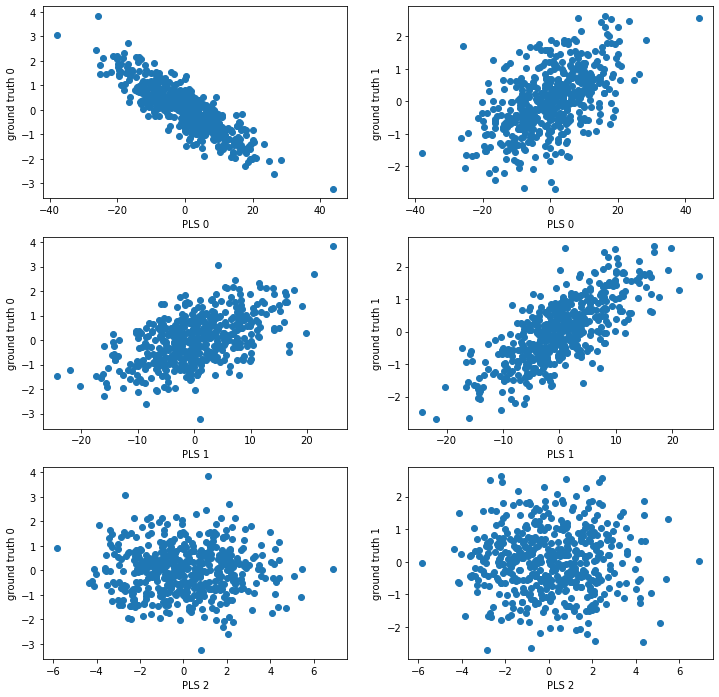
Once that the PLS parameters are estimated, we can solve the regression problem for predicting Y from X. We adopt the scheme used in scikit-learn, where a rotation matrix is first estimated to accoung for non-cummutativity between projection (weights) and reconstruction (loadings).
# Identifying rotation from X to t
# t_x * loadings_x = X
# t_x * loadings_x.T * weight = X * weight
# t_x =  X * weight * (loadings_x.T * weight)^-1 = X * rotations_x

rotations_x = weight_x.dot(np.linalg.pinv(loading_x.T.dot(weight_x)))

# Solving the regression from X to Y
# Y = t_x * loadings_y.T
# Y = X * rotations_x * loadings_y.T

regression_coef = np.dot(rotations_x, loading_y.T)
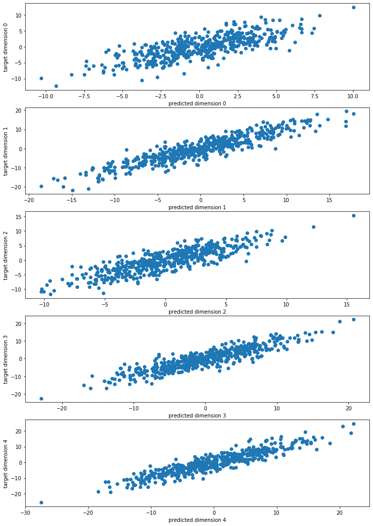
plt.figure(figsize=(12, 18))
for i in range(Y.shape[1]):
  plt.subplot(Y.shape[1], 1, i+1)
  plt.scatter(X.dot(regression_coef)[:,i], Y[:,i])
  plt.xlabel('predicted dimension ' + str(i))
  plt.ylabel('target dimension ' + str(i))
plt.show()
# Comparing with SVD of covariance matrix

eig_val_x, eig_vect, eig_val_y = np.linalg.svd(X.transpose().dot(Y))
print('Eigenvalues for X \n' + str(np.real(eig_val_x[:,:3])))
print('Estimated weights for X\n' + str(np.real(weight_x[:,:3])))
Eigenvalues for X
[[-0.36753226  0.32695545  0.31901594]
 [ 0.54017132 -0.51142438 -0.13635813]
 [-0.73596167 -0.54668695 -0.38095079]
 [ 0.07131382 -0.54068145  0.43213359]
 [ 0.16251074  0.20085364 -0.74011644]]
Estimated weights for X
[[ 0.36753226  0.32695545  0.31901594]
 [-0.54017132 -0.51142438 -0.13635813]
 [ 0.73596167 -0.54668695 -0.38095079]
 [-0.07131382 -0.54068145  0.43213359]
 [-0.16251074  0.20085364 -0.74011644]]
print('Eigenvalues for Y \n' + str(np.real(eig_val_y.T[:,:3])))
print('Estimated weights for Y\n' + str(np.real(weight_y[:,:3])))
Eigenvalues for Y
[[-0.22469208 -0.22321827  0.22848154]
 [ 0.42360052 -0.82303817 -0.17028297]
 [-0.34143196  0.23277327 -0.37414229]
 [ 0.53070486  0.30658588 -0.6691619 ]
 [ 0.60979721  0.35299218  0.57536058]]
Estimated weights for Y
[[ 0.22469208 -0.22321827  0.22848154]
 [-0.42360052 -0.82303817 -0.17028297]
 [ 0.34143196  0.23277327 -0.37414229]
 [-0.53070486  0.30658588 -0.6691619 ]
 [-0.60979721  0.35299218  0.57536058]]
# PLS in scikit-learn

plsca = PLSCanonical(n_components=3, scale = False)
plsca.fit(X, Y)
PLSCanonical(n_components=3, scale=False)
print(plsca.x_weights_)
print(plsca.y_weights_)
[[ 0.36745572 -0.32646087 -0.30267791]
 [-0.5399922   0.51144303  0.11763542]
 [ 0.73610243  0.54625149  0.37318486]
 [-0.07130735  0.54144866 -0.38043117]
 [-0.16264435 -0.20072864  0.78137902]]
[[ 0.22485955  0.22212135 -0.2169345 ]
 [-0.42328296  0.82287418  0.1493648 ]
 [ 0.34172183 -0.23372426  0.32376757]
 [-0.53074024 -0.30704996  0.68434385]
 [-0.60976283 -0.35303468 -0.59789433]]
NIPALS for CCA
import scipy

# Nipals method for CCA

# Defining empty arrays where to store results

# Reconstruction from latent space to data
loading_x_cca = np.ndarray([X.shape[1],n_components])
loading_y_cca = np.ndarray([Y.shape[1],n_components])

# Projections into the latent space
scores_x_cca = np.ndarray([X.shape[0],n_components])
scores_y_cca = np.ndarray([Y.shape[0],n_components])

# Latent variables
weight_x_cca = np.ndarray([X.shape[1],n_components])
weight_y_cca = np.ndarray([Y.shape[1],n_components])

# Initialization of data matrices
current_X = X
current_Y = Y

for i in range(n_components):
    # Initialization of current latent variables as a data column
    t_x = current_X[:,0]

    # NIPALS iterations
    for _ in range(500):
        ## CCA variant
        # estimating Y weights given data Y and latent variables from X
        Y_pinv = np.linalg.pinv(current_Y)
        #Y_pinv = np.linalg.solve(current_Y.dot(current_Y.T),current_Y).T
        w_y = Y_pinv.dot(t_x)

        # normalizing Y weights
        w_y = w_y/np.sqrt(np.sum(w_y**2))
        # estimating latent variables from Y given data Y and Y weights
        t_y = current_Y.dot(w_y)

        ## CCA variant
        # estimating X weights given data X and latent variables from Y
        X_pinv = np.linalg.pinv(current_X)
        #X_pinv = np.linalg.solve(current_X.dot(current_X.T),current_X).T
        w_x = X_pinv.dot(t_y)

        # normalizing X weights
        w_x = w_x/np.sqrt(np.sum(w_x**2))
        # estimating latent variables from X given data X and X weights
        t_x = current_X.dot(w_x)


    # Weights are such that X * weights = t
    weight_x_cca[:,i] = w_x
    weight_y_cca[:,i] = w_y

    # Latent dimensions
    scores_x_cca[:,i] = t_x
    scores_x_cca[:,i] = t_y

    # Loadings obtained by regressing X on t (X = t * loadings)

    loading_x_cca[:,i] = np.dot(current_X.T, t_x)/t_x.transpose().dot(t_x)
    loading_y_cca[:,i] = np.dot(current_Y.T, t_y)/t_y.transpose().dot(t_y)

    # Deflation = current_data - current_reconstruction

    current_X = current_X - t_x.reshape(len(t_x),1).dot(w_x.reshape(1,len(w_x)))
    current_Y = current_Y - t_y.reshape(len(t_y),1).dot(w_x.reshape(1,len(w_y)))
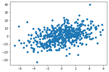
print(weight_x_cca)

plt.scatter(X.dot(weight_x_cca)[:,2], Y.dot(weight_y_cca)[:,2])
[[ 0.24391049  0.36361822  0.79534955]
 [-0.47437693 -0.58135481  0.07701894]
 [ 0.82921211 -0.45865491 -0.17520398]
 [-0.04561038 -0.56190597  0.56872597]
 [-0.16062744  0.06087473 -0.0856826 ]]
<matplotlib.collections.PathCollection at 0x7f7070df44d0>
cca = CCA(n_components=3, scale = False)
cca.fit(X,Y)
print(cca.x_weights_)

plt.scatter(X.dot(weight_x_cca)[:,2], Y.dot(weight_y_cca)[:,2])
[[ 0.2415487  -0.32772785 -0.24927466]
 [-0.47054284  0.58859583  0.10763174]
 [ 0.83233244  0.44252343  0.28013453]
 [-0.04077413  0.58734795 -0.35211385]
 [-0.16063576 -0.07310815  0.85077496]]
<matplotlib.collections.PathCollection at 0x7f7070d38790>

Reduced Rank Regression
We finally review reduced rank regression through eigen-decomposition.
# Reduced Rank Regression

n_components = 2
Gamma = np.eye(n_components)

SYX = np.dot(Y.T,X)

SXX = np.dot(X.T,X)

U, S, V = np.linalg.svd(np.dot(SYX, np.dot(np.linalg.pinv(SXX), SYX.T)))

A = V[0:n_components, :].T

B = np.dot(np.dot(A.T,SYX), np.linalg.pinv(SXX))
A
array([[-0.24936409, -0.19522003],
       [ 0.3233369 , -0.86712778],
       [-0.31172187,  0.27190596],
       [ 0.56300866,  0.2411439 ],
       [ 0.64739595,  0.27909733]])
B
array([[-0.17847633,  0.34992334, -0.88917092, -0.05742634,  0.16716151],
       [ 0.33903723, -0.60088957, -0.58551613, -0.63995952,  0.10694492]])
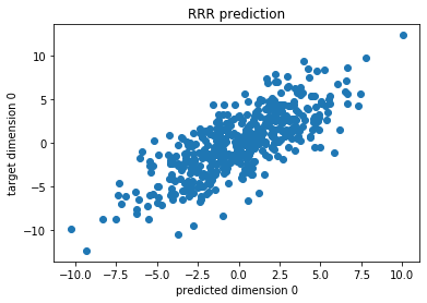
regression_coef_rrr = np.dot(A,B)
plt.scatter(np.dot(X,regression_coef)[:,0],Y[:,0])
plt.xlabel('predicted dimension 0')
plt.ylabel('target dimension 0')
plt.title('RRR prediction')
plt.show()
Sparsity in latent variable models
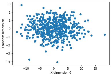
We now focus on the effect of spurious variables in mutivariate models. To explore this new setting, we are going to add spurious random features to our data matrices X and Y.
## Adding 3 random dimensions
## No association is expected from these features

X_ext = np.hstack([X,np.random.randn(n*3).reshape([n,3])])
Y_ext = np.hstack([Y,np.random.randn(n*3).reshape([n,3])])
plt.scatter(X_ext[:,0], Y_ext[:,-1])
plt.xlabel('X dimension 0')
plt.ylabel('Y random dimension')
plt.show()
from sklearn import linear_model

n_components = 3

#### Sparse PLS via regularization in NIPALS [Waaijenborg, et al 2007]
# Everything is as for the standard NIPALS algorithm, with the added sparse estimation step

loading_x_sparse = np.ndarray([X_ext.shape[1],n_components])
loading_y_sparse = np.ndarray([Y_ext.shape[1],n_components])

scores_x_sparse = np.ndarray([X_ext.shape[0],n_components])
scores_y_sparse = np.ndarray([Y_ext.shape[0],n_components])

weight_x_sparse = np.ndarray([X_ext.shape[1],n_components])
weight_y_sparse = np.ndarray([Y_ext.shape[1],n_components])

current_X = X_ext
current_Y = Y_ext

## Penalty parameter for regularization
penalty = 10

eps = 1e-4

for i in range(n_components):
    t_x = current_X[:,0]
    for _ in range(100):
        w_y = current_Y.transpose().dot(t_x)/(t_x.transpose().dot(t_x))
        w_y = w_y/np.sqrt(np.sum(w_y**2))
        t_y = current_Y.dot(w_y)
        w_x = current_X.transpose().dot(t_y)/(t_y.transpose().dot(t_y))
        w_x = w_x/np.sqrt(np.sum(w_x**2))
        t_x = current_X.dot(w_x)

        ## Estimating sparse model for the weights of X
        lasso_x = linear_model.Lasso(alpha = penalty)
        lasso_x.fit(t_x.reshape(-1, 1), current_X)

        ## Estimating sparse model for the weights of Y
        lasso_y = linear_model.Lasso(alpha = penalty)
        lasso_y.fit(t_y.reshape(-1, 1), current_Y)

        # Replacing the original weights with the sparse estimation
        w_x = (lasso_x.coef_ / (np.sqrt(np.sum(lasso_x.coef_**2) + eps))).reshape([X_ext.shape[1]])
        w_y = (lasso_y.coef_ / (np.sqrt(np.sum(lasso_y.coef_**2) + eps))).reshape([Y_ext.shape[1]])

    # Weights are such that X * weights = t
    weight_x_sparse[:,i] = w_x
    weight_y_sparse[:,i] = w_y

    # Latent dimensions
    scores_x_sparse[:,i] = t_x
    scores_x_sparse[:,i] = t_y

    # Loadings obtained by regressing X on t (X = t * loadings)

    loading_x_sparse[:,i] = np.dot(current_X.T, t_x)/t_x.transpose().dot(t_x)
    loading_y_sparse[:,i] = np.dot(current_Y.T, t_y)/t_y.transpose().dot(t_y)

    # Deflation

    current_X = current_X - t_x.reshape(len(t_x),1).dot(w_x.reshape(1,len(w_x)))
    current_Y = current_Y - t_y.reshape(len(t_y),1).dot(w_y.reshape(1,len(w_y)))
We observe that the new weights are similar to the ones estimated before. However the parameters associated with the spurious dimension are entirely set to zero. This indicates that the model does not find these features necessary to explain the common variability between X and Y. There are also other weights which are set to zero, corresponding to the third latent dimension. This makes sense, as our synthetic data was indeed created with only two latent dimensions.
weight_x_sparse
array([[ 0.35947916,  0.09613335,  0.        ],
       [-0.57208323, -0.5017898 ,  0.        ],
       [ 0.73260855, -0.60111564,  0.        ],
       [-0.01764855, -0.61404951,  0.        ],
       [-0.0795538 ,  0.        ,  0.        ],
       [ 0.        ,  0.        ,  0.        ],
       [ 0.        ,  0.        ,  0.        ],
       [ 0.        ,  0.        , -0.        ]])
weight_y_sparse
array([[ 0.19008698, -0.03395428, -0.        ],
       [-0.3361836 , -0.95121052,  0.        ],
       [ 0.29093832,  0.05788278,  0.        ],
       [-0.56391994,  0.17865107,  0.        ],
       [-0.66936112,  0.24197983,  0.        ],
       [-0.        , -0.        , -0.        ],
       [ 0.        , -0.        , -0.        ],
       [-0.        , -0.        , -0.        ]])
## Non-sparse parameters previously estimated

print(weight_x)
print(weight_y)
[[ 0.36753226  0.32695545  0.31901594]
 [-0.54017132 -0.51142438 -0.13635813]
 [ 0.73596167 -0.54668695 -0.38095079]
 [-0.07131382 -0.54068145  0.43213359]
 [-0.16251074  0.20085364 -0.74011644]]
[[ 0.22469208 -0.22321827  0.22848154]
 [-0.42360052 -0.82303817 -0.17028297]
 [ 0.34143196  0.23277327 -0.37414229]
 [-0.53070486  0.30658588 -0.6691619 ]
 [-0.60979721  0.35299218  0.57536058]]
## PLS result from scikit-learn PLS on the data augmented with spurious dimensions

plsca = PLSCanonical(n_components=3, scale = False)
plsca.fit(X_ext, Y_ext)
print(plsca.x_weights_)
print(plsca.y_weights_)
[[ 0.36744392 -0.32636735 -0.3736012 ]
 [-0.53999014  0.51133222  0.13293972]
 [ 0.73606624  0.54628291  0.34582048]
 [-0.07131057  0.54141809 -0.49749784]
 [-0.16262691 -0.20075143  0.52023542]
 [ 0.00653338 -0.00825341  0.39402462]
 [ 0.00339241 -0.00798747  0.07331524]
 [ 0.0038984  -0.00566521  0.21066051]]
[[ 0.22481823  0.22219588 -0.39318404]
 [-0.4232868   0.82282067  0.19587236]
 [ 0.34171379 -0.2337191   0.39240653]
 [-0.53068906 -0.30708105  0.46282095]
 [-0.6097158  -0.353037   -0.46080397]
 [-0.00986828  0.00097623 -0.2131351 ]
 [ 0.00469737  0.00268147 -0.28959681]
 [-0.00361132  0.00533588 -0.31180287]]
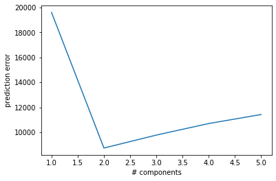
Cross-validating components
In addition to sparsity, the optimal number of components in latent variable models can be identified by cross-validation. A common strategy is to train the model on a subset of the data and to quantify the predicted residual error sum of squares (PRESS) in non-overlapping testing data. We can finally choose the number of latent dimensions leading to the lowest average PRESS.
n_cross_valid_run = 200

# max number of components to test
n_components = 5

rep_results = []
for i in range(n_components):
   rep_results.append([])

for k in range(n_components):
  for i in range(n_cross_valid_run):

    # Sampling disjoint set of indices for splitting the data
    batch1_idx = np.random.choice(range(X_ext.shape[0]), size = int(X_ext.shape[0]/2), replace = False)
    batch2_idx = np.where(np.in1d(range(X_ext.shape[0]), batch1_idx, assume_unique=True, invert = True))[0]

    # Creating independent data batches for X
    X_1 = X_ext[batch1_idx, :]
    X_2 = X_ext[batch2_idx, :]

    # Creating independent data batches for Y
    Y_1 = Y_ext[batch1_idx, :]
    Y_2 = Y_ext[batch2_idx, :]

    # Creating a model for each data batch
    plsca1 = PLSCanonical(n_components = k+1, scale = False)
    plsca2 = PLSCanonical(n_components = k+1, scale = False)

    # Fitting a model for each data batch
    plsca1.fit(X_1,Y_1)
    plsca2.fit(X_2,Y_2)

    # Quantifying the prediction error on the unseen data batch
    err1 = np.sum((plsca1.predict(X_2) - Y_2)**2)
    err2 = np.sum((plsca2.predict(X_1) - Y_1)**2)

    rep_results[k].append(np.mean([err1,err2]))
plt.plot(range(1,n_components+1),np.mean(rep_results, 1))
plt.xlabel('# components')
plt.ylabel('prediction error')
plt.show()
Multi-channel Variational Autoencoder
The last part of this tutorial concerns the use of the multi-channel variational autoencoder (https://gitlab.inria.fr/epione_ML/mcvae), a more advanced methods for the joint analysis and prediction of several modalities.
VAE
The Variational Autoencoer is a latent variable model composed by one encoder and one decoder associated to a single channel. The latent distribution and the decoding distribution are implemented as follows:
They are Gaussians with moments parametrized by Neural Networks (or a linear transformation layer in a simple case).

Exercise
Why is convenient to use \(\log\) values for the parametrization the variance networks output (W_logvar, W_out_logvar)?
Sparse VAE
To favour sparsity in the latent space we implement the latent distribution as follows:
where:
Tha parameter \(\alpha_i\) represents the odds of pruning the \(i\)-th latent dimension according to:

MCVAE
The MultiChannel VAE is built by stacking multiple VAEs and allowing the decoding distributions to be computed from every input channel.

Exercise
Sketch the Sparse MCVAE with 3 channels. [Solution]
![[Solution]](https://gitlab.inria.fr/epione/flhd/-/raw/master/heterogeneous_data/img/sparse_mcvae_3ch.svg)
import torch
from mcvae.models import Mcvae
from mcvae.models.utils import DEVICE, load_or_fit
from mcvae.diagnostics import *
from mcvae.plot import lsplom

print(f"Running on {DEVICE}")  # cpu or gpu

FORCE_REFIT = False  # Set this to 'True' if ou want to refit the models instead of loading them from file.
Running on cpu
### To initialization of the mcvae model you should provide:

# 1 - a list with the different data channels
data = [X, Y]
data = [torch.Tensor(_) for _ in data]  #warning: data matrices must be converted to type torch.Tensor

# 1 - a dictionary with the data and model characteristics
init_dict = {
    'data': data,
    'lat_dim': n_components,
}
# Here we initialize an instance of the model

# Multi-Channel VAE
torch.manual_seed(24)
model = Mcvae(**init_dict)
model.to(DEVICE)
print(model)
Mcvae(
  (vae): ModuleList(
    (0): VAE(
      (W_out_logvar): Parameter(shape=torch.Size([1, 5]))
      (W_mu): Linear(in_features=5, out_features=5, bias=True)
      (W_logvar): Linear(in_features=5, out_features=5, bias=True)
      (W_out): Linear(in_features=5, out_features=5, bias=True)
    )
    (1): VAE(
      (W_out_logvar): Parameter(shape=torch.Size([1, 5]))
      (W_mu): Linear(in_features=5, out_features=5, bias=True)
      (W_logvar): Linear(in_features=5, out_features=5, bias=True)
      (W_out): Linear(in_features=5, out_features=5, bias=True)
    )
  )
)
###################
## Model Fitting ##
###################

# Set up the optimizer
adam_lr = 1e-2
n_epochs = 5000
model.optimizer = torch.optim.Adam(model.parameters(), lr=adam_lr)

# We will use the custom routine "load_or_fit" to fit the model
help(load_or_fit)
Help on function load_or_fit in module mcvae.models.utils:

load_or_fit(model, data, epochs, ptfile, init_loss=True, minibatch=False, force_fit=False)
    Routine to train or load a model.
    :param model: model to optimize
    :param data: training data
    :param epochs: number of training epochs
    :param ptfile: path to *.pt file where to save the trained model
    :param force_fit: force the training even if the model is already trained
# Fit the model
load_or_fit(model=model, data=data, epochs=n_epochs, ptfile='model.pt', force_fit=True)
	Creating model.pt.running
	Created: 2021-01-08 18:02:05.267851
Start fitting: 2021-01-08 18:02:05.268239
	Model destination: model.pt
====> Epoch:    0/5000 (0%)	Loss: 4262660.5000	LL: -1298590.0000	KL: 2964070.5000	LL/KL: -0.4381
====> Epoch:   10/5000 (0%)	Loss: 43945.0391	LL: -34668.4375	KL: 9276.6035	LL/KL: -3.7372
====> Epoch:   20/5000 (0%)	Loss: 19446.6035	LL: -17842.4414	KL: 1604.1619	LL/KL: -11.1226
====> Epoch:   30/5000 (1%)	Loss: 12697.3916	LL: -11797.3516	KL: 900.0399	LL/KL: -13.1076
====> Epoch:   40/5000 (1%)	Loss: 6696.4473	LL: -5948.7456	KL: 747.7017	LL/KL: -7.9560
====> Epoch:   50/5000 (1%)	Loss: 14101.9600	LL: -13389.3281	KL: 712.6315	LL/KL: -18.7886
====> Epoch:   60/5000 (1%)	Loss: 6858.8511	LL: -6148.5029	KL: 710.3480	LL/KL: -8.6556
====> Epoch:   70/5000 (1%)	Loss: 7487.5254	LL: -6770.8442	KL: 716.6814	LL/KL: -9.4475
====> Epoch:   80/5000 (2%)	Loss: 3859.8472	LL: -3138.4307	KL: 721.4165	LL/KL: -4.3504
====> Epoch:   90/5000 (2%)	Loss: 4518.0630	LL: -3797.2717	KL: 720.7911	LL/KL: -5.2682
====> Epoch:  100/5000 (2%)	Loss: 5719.1602	LL: -5000.9023	KL: 718.2576	LL/KL: -6.9625
====> Epoch:  110/5000 (2%)	Loss: 2709.6421	LL: -1994.7473	KL: 714.8947	LL/KL: -2.7903
====> Epoch:  120/5000 (2%)	Loss: 7239.8066	LL: -6530.8994	KL: 708.9070	LL/KL: -9.2126
====> Epoch:  130/5000 (3%)	Loss: 2872.6157	LL: -2171.9895	KL: 700.6263	LL/KL: -3.1001
====> Epoch:  140/5000 (3%)	Loss: 2293.5227	LL: -1601.2192	KL: 692.3034	LL/KL: -2.3129
====> Epoch:  150/5000 (3%)	Loss: 6731.0962	LL: -6047.7144	KL: 683.3818	LL/KL: -8.8497
====> Epoch:  160/5000 (3%)	Loss: 3181.1064	LL: -2508.8794	KL: 672.2271	LL/KL: -3.7322
====> Epoch:  170/5000 (3%)	Loss: 6107.2334	LL: -5445.0718	KL: 662.1615	LL/KL: -8.2232
====> Epoch:  180/5000 (4%)	Loss: 4395.3936	LL: -3742.2568	KL: 653.1368	LL/KL: -5.7297
====> Epoch:  190/5000 (4%)	Loss: 2763.1292	LL: -2120.5781	KL: 642.5511	LL/KL: -3.3002
====> Epoch:  200/5000 (4%)	Loss: 2477.9043	LL: -1844.8848	KL: 633.0195	LL/KL: -2.9144
====> Epoch:  210/5000 (4%)	Loss: 2105.9983	LL: -1484.8384	KL: 621.1599	LL/KL: -2.3904
====> Epoch:  220/5000 (4%)	Loss: 13323.0703	LL: -12711.7891	KL: 611.2809	LL/KL: -20.7953
====> Epoch:  230/5000 (5%)	Loss: 5057.8389	LL: -4457.0781	KL: 600.7610	LL/KL: -7.4191
====> Epoch:  240/5000 (5%)	Loss: 4228.7827	LL: -3635.3999	KL: 593.3828	LL/KL: -6.1266
====> Epoch:  250/5000 (5%)	Loss: 3765.3745	LL: -3181.7815	KL: 583.5930	LL/KL: -5.4521
====> Epoch:  260/5000 (5%)	Loss: 3960.7463	LL: -3385.7822	KL: 574.9642	LL/KL: -5.8887
====> Epoch:  270/5000 (5%)	Loss: 2081.4968	LL: -1515.2067	KL: 566.2901	LL/KL: -2.6757
====> Epoch:  280/5000 (6%)	Loss: 6944.0654	LL: -6382.9033	KL: 561.1620	LL/KL: -11.3744
====> Epoch:  290/5000 (6%)	Loss: 3887.6899	LL: -3335.7651	KL: 551.9247	LL/KL: -6.0439
====> Epoch:  300/5000 (6%)	Loss: 3377.1025	LL: -2831.6406	KL: 545.4619	LL/KL: -5.1913
====> Epoch:  310/5000 (6%)	Loss: 3452.5525	LL: -2914.7649	KL: 537.7876	LL/KL: -5.4199
====> Epoch:  320/5000 (6%)	Loss: 2786.2290	LL: -2257.6572	KL: 528.5719	LL/KL: -4.2712
====> Epoch:  330/5000 (7%)	Loss: 1775.6956	LL: -1252.7754	KL: 522.9201	LL/KL: -2.3957
====> Epoch:  340/5000 (7%)	Loss: 3147.1799	LL: -2630.1743	KL: 517.0056	LL/KL: -5.0873
====> Epoch:  350/5000 (7%)	Loss: 2116.6458	LL: -1609.1597	KL: 507.4861	LL/KL: -3.1708
====> Epoch:  360/5000 (7%)	Loss: 3679.0774	LL: -3177.3794	KL: 501.6980	LL/KL: -6.3333
====> Epoch:  370/5000 (7%)	Loss: 2289.3469	LL: -1792.4320	KL: 496.9149	LL/KL: -3.6071
====> Epoch:  380/5000 (8%)	Loss: 3934.2031	LL: -3446.0605	KL: 488.1425	LL/KL: -7.0595
====> Epoch:  390/5000 (8%)	Loss: 2178.9221	LL: -1699.2437	KL: 479.6784	LL/KL: -3.5425
====> Epoch:  400/5000 (8%)	Loss: 3150.6499	LL: -2679.0728	KL: 471.5771	LL/KL: -5.6811
====> Epoch:  410/5000 (8%)	Loss: 2006.5717	LL: -1541.8043	KL: 464.7673	LL/KL: -3.3174
====> Epoch:  420/5000 (8%)	Loss: 2842.1255	LL: -2385.0315	KL: 457.0941	LL/KL: -5.2178
====> Epoch:  430/5000 (9%)	Loss: 2685.0171	LL: -2235.1396	KL: 449.8773	LL/KL: -4.9683
====> Epoch:  440/5000 (9%)	Loss: 3580.0781	LL: -3133.2732	KL: 446.8050	LL/KL: -7.0126
====> Epoch:  450/5000 (9%)	Loss: 2881.6396	LL: -2439.3345	KL: 442.3052	LL/KL: -5.5150
====> Epoch:  460/5000 (9%)	Loss: 3728.0725	LL: -3290.8694	KL: 437.2030	LL/KL: -7.5271
====> Epoch:  470/5000 (9%)	Loss: 2724.9758	LL: -2292.2390	KL: 432.7368	LL/KL: -5.2971
====> Epoch:  480/5000 (10%)	Loss: 2711.6714	LL: -2287.2346	KL: 424.4366	LL/KL: -5.3889
====> Epoch:  490/5000 (10%)	Loss: 1880.4370	LL: -1461.4816	KL: 418.9554	LL/KL: -3.4884
====> Epoch:  500/5000 (10%)	Loss: 2494.4944	LL: -2080.9089	KL: 413.5854	LL/KL: -5.0314
====> Epoch:  510/5000 (10%)	Loss: 1736.9312	LL: -1324.5104	KL: 412.4208	LL/KL: -3.2116
====> Epoch:  520/5000 (10%)	Loss: 2838.1016	LL: -2429.9229	KL: 408.1786	LL/KL: -5.9531
====> Epoch:  530/5000 (11%)	Loss: 3567.1365	LL: -3164.5684	KL: 402.5682	LL/KL: -7.8610
====> Epoch:  540/5000 (11%)	Loss: 1835.9888	LL: -1439.1138	KL: 396.8751	LL/KL: -3.6261
====> Epoch:  550/5000 (11%)	Loss: 2106.6096	LL: -1714.1101	KL: 392.4995	LL/KL: -4.3672
====> Epoch:  560/5000 (11%)	Loss: 1757.2501	LL: -1368.5223	KL: 388.7278	LL/KL: -3.5205
====> Epoch:  570/5000 (11%)	Loss: 1735.3756	LL: -1351.3695	KL: 384.0061	LL/KL: -3.5191
====> Epoch:  580/5000 (12%)	Loss: 1979.7140	LL: -1599.3445	KL: 380.3695	LL/KL: -4.2047
====> Epoch:  590/5000 (12%)	Loss: 2113.2715	LL: -1738.4941	KL: 374.7774	LL/KL: -4.6387
====> Epoch:  600/5000 (12%)	Loss: 1582.7756	LL: -1211.4095	KL: 371.3661	LL/KL: -3.2620
====> Epoch:  610/5000 (12%)	Loss: 2550.9966	LL: -2183.7983	KL: 367.1982	LL/KL: -5.9472
====> Epoch:  620/5000 (12%)	Loss: 3524.0396	LL: -3160.2539	KL: 363.7857	LL/KL: -8.6871
====> Epoch:  630/5000 (13%)	Loss: 2121.2957	LL: -1763.3776	KL: 357.9180	LL/KL: -4.9268
====> Epoch:  640/5000 (13%)	Loss: 1560.4982	LL: -1205.3318	KL: 355.1664	LL/KL: -3.3937
====> Epoch:  650/5000 (13%)	Loss: 2421.0500	LL: -2070.0435	KL: 351.0065	LL/KL: -5.8975
====> Epoch:  660/5000 (13%)	Loss: 2265.9092	LL: -1918.2366	KL: 347.6726	LL/KL: -5.5174
====> Epoch:  670/5000 (13%)	Loss: 1571.7317	LL: -1226.0120	KL: 345.7198	LL/KL: -3.5463
====> Epoch:  680/5000 (14%)	Loss: 4609.3799	LL: -4268.1899	KL: 341.1900	LL/KL: -12.5097
====> Epoch:  690/5000 (14%)	Loss: 1591.5065	LL: -1255.7960	KL: 335.7104	LL/KL: -3.7407
====> Epoch:  700/5000 (14%)	Loss: 3109.3455	LL: -2776.6707	KL: 332.6749	LL/KL: -8.3465
====> Epoch:  710/5000 (14%)	Loss: 1970.4255	LL: -1642.4529	KL: 327.9727	LL/KL: -5.0079
====> Epoch:  720/5000 (14%)	Loss: 1787.7649	LL: -1462.7594	KL: 325.0055	LL/KL: -4.5007
====> Epoch:  730/5000 (15%)	Loss: 2275.4277	LL: -1952.7251	KL: 322.7026	LL/KL: -6.0512
====> Epoch:  740/5000 (15%)	Loss: 2411.7817	LL: -2093.2559	KL: 318.5259	LL/KL: -6.5717
====> Epoch:  750/5000 (15%)	Loss: 2171.4382	LL: -1856.8210	KL: 314.6172	LL/KL: -5.9018
====> Epoch:  760/5000 (15%)	Loss: 1972.3674	LL: -1660.2032	KL: 312.1642	LL/KL: -5.3184
====> Epoch:  770/5000 (15%)	Loss: 1599.5530	LL: -1289.0352	KL: 310.5179	LL/KL: -4.1512
====> Epoch:  780/5000 (16%)	Loss: 1588.9763	LL: -1282.9235	KL: 306.0529	LL/KL: -4.1918
====> Epoch:  790/5000 (16%)	Loss: 1825.2235	LL: -1524.0449	KL: 301.1786	LL/KL: -5.0603
====> Epoch:  800/5000 (16%)	Loss: 2668.4998	LL: -2369.5227	KL: 298.9771	LL/KL: -7.9254
====> Epoch:  810/5000 (16%)	Loss: 2814.1914	LL: -2516.2664	KL: 297.9249	LL/KL: -8.4460
====> Epoch:  820/5000 (16%)	Loss: 1627.4493	LL: -1334.5055	KL: 292.9438	LL/KL: -4.5555
====> Epoch:  830/5000 (17%)	Loss: 1940.0685	LL: -1649.6368	KL: 290.4317	LL/KL: -5.6799
====> Epoch:  840/5000 (17%)	Loss: 2364.3738	LL: -2075.8496	KL: 288.5241	LL/KL: -7.1947
====> Epoch:  850/5000 (17%)	Loss: 1524.1296	LL: -1236.8584	KL: 287.2712	LL/KL: -4.3055
====> Epoch:  860/5000 (17%)	Loss: 1875.9878	LL: -1594.3328	KL: 281.6550	LL/KL: -5.6606
====> Epoch:  870/5000 (17%)	Loss: 1628.6495	LL: -1348.7826	KL: 279.8669	LL/KL: -4.8194
====> Epoch:  880/5000 (18%)	Loss: 1761.2710	LL: -1481.9734	KL: 279.2976	LL/KL: -5.3061
====> Epoch:  890/5000 (18%)	Loss: 3350.5596	LL: -3075.5371	KL: 275.0224	LL/KL: -11.1829
====> Epoch:  900/5000 (18%)	Loss: 2062.5210	LL: -1790.2250	KL: 272.2959	LL/KL: -6.5746
====> Epoch:  910/5000 (18%)	Loss: 2666.9690	LL: -2398.1233	KL: 268.8458	LL/KL: -8.9201
====> Epoch:  920/5000 (18%)	Loss: 1707.1511	LL: -1441.3044	KL: 265.8467	LL/KL: -5.4216
====> Epoch:  930/5000 (19%)	Loss: 1457.5961	LL: -1192.8110	KL: 264.7851	LL/KL: -4.5048
====> Epoch:  940/5000 (19%)	Loss: 2139.0674	LL: -1878.0316	KL: 261.0356	LL/KL: -7.1945
====> Epoch:  950/5000 (19%)	Loss: 2519.4126	LL: -2258.8013	KL: 260.6112	LL/KL: -8.6673
====> Epoch:  960/5000 (19%)	Loss: 2455.6077	LL: -2196.4492	KL: 259.1585	LL/KL: -8.4753
====> Epoch:  970/5000 (19%)	Loss: 1682.2816	LL: -1428.2273	KL: 254.0543	LL/KL: -5.6217
====> Epoch:  980/5000 (20%)	Loss: 1229.0485	LL: -975.1719	KL: 253.8765	LL/KL: -3.8411
====> Epoch:  990/5000 (20%)	Loss: 1272.7069	LL: -1023.4662	KL: 249.2407	LL/KL: -4.1063
====> Epoch: 1000/5000 (20%)	Loss: 2016.0963	LL: -1769.5736	KL: 246.5227	LL/KL: -7.1781
====> Epoch: 1010/5000 (20%)	Loss: 1465.2620	LL: -1219.1506	KL: 246.1114	LL/KL: -4.9537
====> Epoch: 1020/5000 (20%)	Loss: 1232.1704	LL: -988.1989	KL: 243.9716	LL/KL: -4.0505
====> Epoch: 1030/5000 (21%)	Loss: 1321.5819	LL: -1079.4614	KL: 242.1205	LL/KL: -4.4584
====> Epoch: 1040/5000 (21%)	Loss: 3451.2773	LL: -3211.1797	KL: 240.0978	LL/KL: -13.3745
====> Epoch: 1050/5000 (21%)	Loss: 1498.3079	LL: -1260.6826	KL: 237.6252	LL/KL: -5.3053
====> Epoch: 1060/5000 (21%)	Loss: 2068.7151	LL: -1832.0361	KL: 236.6789	LL/KL: -7.7406
====> Epoch: 1070/5000 (21%)	Loss: 1710.2220	LL: -1476.9397	KL: 233.2823	LL/KL: -6.3311
====> Epoch: 1080/5000 (22%)	Loss: 1126.5889	LL: -894.3732	KL: 232.2156	LL/KL: -3.8515
====> Epoch: 1090/5000 (22%)	Loss: 2401.8350	LL: -2169.5151	KL: 232.3199	LL/KL: -9.3385
====> Epoch: 1100/5000 (22%)	Loss: 2254.7361	LL: -2026.5315	KL: 228.2046	LL/KL: -8.8803
====> Epoch: 1110/5000 (22%)	Loss: 1205.6593	LL: -977.9169	KL: 227.7423	LL/KL: -4.2940
====> Epoch: 1120/5000 (22%)	Loss: 1547.9728	LL: -1322.4303	KL: 225.5425	LL/KL: -5.8633
====> Epoch: 1130/5000 (23%)	Loss: 1492.6935	LL: -1270.3347	KL: 222.3587	LL/KL: -5.7130
====> Epoch: 1140/5000 (23%)	Loss: 2329.0613	LL: -2105.9451	KL: 223.1162	LL/KL: -9.4388
====> Epoch: 1150/5000 (23%)	Loss: 1332.1718	LL: -1112.1809	KL: 219.9908	LL/KL: -5.0556
====> Epoch: 1160/5000 (23%)	Loss: 1134.4077	LL: -917.7589	KL: 216.6489	LL/KL: -4.2362
====> Epoch: 1170/5000 (23%)	Loss: 2556.1628	LL: -2340.0276	KL: 216.1352	LL/KL: -10.8267
====> Epoch: 1180/5000 (24%)	Loss: 2171.3357	LL: -1957.7233	KL: 213.6124	LL/KL: -9.1648
====> Epoch: 1190/5000 (24%)	Loss: 1463.3451	LL: -1251.0682	KL: 212.2769	LL/KL: -5.8936
====> Epoch: 1200/5000 (24%)	Loss: 1966.2485	LL: -1756.8313	KL: 209.4172	LL/KL: -8.3891
====> Epoch: 1210/5000 (24%)	Loss: 1936.5503	LL: -1729.0808	KL: 207.4695	LL/KL: -8.3341
====> Epoch: 1220/5000 (24%)	Loss: 1112.4226	LL: -904.4305	KL: 207.9921	LL/KL: -4.3484
====> Epoch: 1230/5000 (25%)	Loss: 1140.7767	LL: -936.2104	KL: 204.5663	LL/KL: -4.5766
====> Epoch: 1240/5000 (25%)	Loss: 1180.8647	LL: -977.3467	KL: 203.5181	LL/KL: -4.8023
====> Epoch: 1250/5000 (25%)	Loss: 1231.2023	LL: -1028.8901	KL: 202.3122	LL/KL: -5.0857
====> Epoch: 1260/5000 (25%)	Loss: 1255.2245	LL: -1054.3956	KL: 200.8289	LL/KL: -5.2502
====> Epoch: 1270/5000 (25%)	Loss: 1271.5682	LL: -1072.6709	KL: 198.8973	LL/KL: -5.3931
====> Epoch: 1280/5000 (26%)	Loss: 1317.8157	LL: -1120.7584	KL: 197.0573	LL/KL: -5.6875
====> Epoch: 1290/5000 (26%)	Loss: 1179.8812	LL: -984.6975	KL: 195.1837	LL/KL: -5.0450
====> Epoch: 1300/5000 (26%)	Loss: 1040.5862	LL: -846.2059	KL: 194.3803	LL/KL: -4.3534
====> Epoch: 1310/5000 (26%)	Loss: 1151.3981	LL: -958.2407	KL: 193.1574	LL/KL: -4.9609
====> Epoch: 1320/5000 (26%)	Loss: 1460.1351	LL: -1268.0066	KL: 192.1286	LL/KL: -6.5998
====> Epoch: 1330/5000 (27%)	Loss: 1186.6499	LL: -996.7165	KL: 189.9334	LL/KL: -5.2477
====> Epoch: 1340/5000 (27%)	Loss: 1259.4811	LL: -1069.1423	KL: 190.3388	LL/KL: -5.6170
====> Epoch: 1350/5000 (27%)	Loss: 1281.3859	LL: -1092.9219	KL: 188.4640	LL/KL: -5.7991
====> Epoch: 1360/5000 (27%)	Loss: 1176.5123	LL: -990.7215	KL: 185.7908	LL/KL: -5.3325
====> Epoch: 1370/5000 (27%)	Loss: 2040.7468	LL: -1854.4304	KL: 186.3164	LL/KL: -9.9531
====> Epoch: 1380/5000 (28%)	Loss: 1331.0305	LL: -1146.7010	KL: 184.3295	LL/KL: -6.2209
====> Epoch: 1390/5000 (28%)	Loss: 1434.0869	LL: -1249.6487	KL: 184.4382	LL/KL: -6.7754
====> Epoch: 1400/5000 (28%)	Loss: 1721.0398	LL: -1539.9001	KL: 181.1397	LL/KL: -8.5012
====> Epoch: 1410/5000 (28%)	Loss: 1440.5950	LL: -1259.7344	KL: 180.8607	LL/KL: -6.9652
====> Epoch: 1420/5000 (28%)	Loss: 1870.1147	LL: -1690.8724	KL: 179.2423	LL/KL: -9.4334
====> Epoch: 1430/5000 (29%)	Loss: 1146.2024	LL: -968.6732	KL: 177.5292	LL/KL: -5.4564
====> Epoch: 1440/5000 (29%)	Loss: 1291.2157	LL: -1114.5911	KL: 176.6246	LL/KL: -6.3105
====> Epoch: 1450/5000 (29%)	Loss: 1167.1429	LL: -992.8992	KL: 174.2438	LL/KL: -5.6983
====> Epoch: 1460/5000 (29%)	Loss: 1541.9700	LL: -1368.6398	KL: 173.3302	LL/KL: -7.8961
====> Epoch: 1470/5000 (29%)	Loss: 1334.2880	LL: -1160.0168	KL: 174.2711	LL/KL: -6.6564
====> Epoch: 1480/5000 (30%)	Loss: 1559.2811	LL: -1387.6062	KL: 171.6749	LL/KL: -8.0828
====> Epoch: 1490/5000 (30%)	Loss: 1385.4377	LL: -1215.6008	KL: 169.8369	LL/KL: -7.1575
====> Epoch: 1500/5000 (30%)	Loss: 2009.4011	LL: -1839.0745	KL: 170.3267	LL/KL: -10.7973
====> Epoch: 1510/5000 (30%)	Loss: 1121.4117	LL: -953.1074	KL: 168.3044	LL/KL: -5.6630
====> Epoch: 1520/5000 (30%)	Loss: 2043.5652	LL: -1876.7042	KL: 166.8610	LL/KL: -11.2471
====> Epoch: 1530/5000 (31%)	Loss: 1153.7765	LL: -988.9729	KL: 164.8036	LL/KL: -6.0009
====> Epoch: 1540/5000 (31%)	Loss: 2205.5872	LL: -2042.0969	KL: 163.4903	LL/KL: -12.4906
====> Epoch: 1550/5000 (31%)	Loss: 1116.8275	LL: -953.1720	KL: 163.6555	LL/KL: -5.8243
====> Epoch: 1560/5000 (31%)	Loss: 1190.0483	LL: -1028.2065	KL: 161.8418	LL/KL: -6.3532
====> Epoch: 1570/5000 (31%)	Loss: 1283.1998	LL: -1121.2623	KL: 161.9375	LL/KL: -6.9240
====> Epoch: 1580/5000 (32%)	Loss: 1140.5878	LL: -979.8543	KL: 160.7335	LL/KL: -6.0961
====> Epoch: 1590/5000 (32%)	Loss: 1143.3615	LL: -984.2577	KL: 159.1038	LL/KL: -6.1863
====> Epoch: 1600/5000 (32%)	Loss: 1675.2139	LL: -1516.7173	KL: 158.4965	LL/KL: -9.5694
====> Epoch: 1610/5000 (32%)	Loss: 1085.5797	LL: -927.8647	KL: 157.7150	LL/KL: -5.8832
====> Epoch: 1620/5000 (32%)	Loss: 1090.6754	LL: -934.8406	KL: 155.8348	LL/KL: -5.9989
====> Epoch: 1630/5000 (33%)	Loss: 866.0853	LL: -710.2181	KL: 155.8672	LL/KL: -4.5566
====> Epoch: 1640/5000 (33%)	Loss: 1217.4338	LL: -1061.5758	KL: 155.8581	LL/KL: -6.8112
====> Epoch: 1650/5000 (33%)	Loss: 915.8037	LL: -762.0650	KL: 153.7387	LL/KL: -4.9569
====> Epoch: 1660/5000 (33%)	Loss: 946.9049	LL: -793.6376	KL: 153.2673	LL/KL: -5.1781
====> Epoch: 1670/5000 (33%)	Loss: 1101.5500	LL: -950.2353	KL: 151.3148	LL/KL: -6.2799
====> Epoch: 1680/5000 (34%)	Loss: 1153.0992	LL: -1001.4298	KL: 151.6694	LL/KL: -6.6027
====> Epoch: 1690/5000 (34%)	Loss: 1225.5017	LL: -1074.3660	KL: 151.1357	LL/KL: -7.1086
====> Epoch: 1700/5000 (34%)	Loss: 972.7237	LL: -823.2496	KL: 149.4741	LL/KL: -5.5076
====> Epoch: 1710/5000 (34%)	Loss: 937.8472	LL: -788.2142	KL: 149.6330	LL/KL: -5.2676
====> Epoch: 1720/5000 (34%)	Loss: 1087.0841	LL: -941.2687	KL: 145.8153	LL/KL: -6.4552
====> Epoch: 1730/5000 (35%)	Loss: 1199.5356	LL: -1052.0037	KL: 147.5320	LL/KL: -7.1307
====> Epoch: 1740/5000 (35%)	Loss: 951.2284	LL: -805.0386	KL: 146.1898	LL/KL: -5.5068
====> Epoch: 1750/5000 (35%)	Loss: 982.2732	LL: -836.9806	KL: 145.2926	LL/KL: -5.7607
====> Epoch: 1760/5000 (35%)	Loss: 1210.2473	LL: -1065.9546	KL: 144.2927	LL/KL: -7.3874
====> Epoch: 1770/5000 (35%)	Loss: 902.0007	LL: -758.2146	KL: 143.7861	LL/KL: -5.2732
====> Epoch: 1780/5000 (36%)	Loss: 1000.2294	LL: -858.0259	KL: 142.2035	LL/KL: -6.0338
====> Epoch: 1790/5000 (36%)	Loss: 989.3272	LL: -847.5911	KL: 141.7361	LL/KL: -5.9801
====> Epoch: 1800/5000 (36%)	Loss: 1184.1068	LL: -1042.6858	KL: 141.4210	LL/KL: -7.3729
====> Epoch: 1810/5000 (36%)	Loss: 987.6963	LL: -847.6875	KL: 140.0088	LL/KL: -6.0545
====> Epoch: 1820/5000 (36%)	Loss: 1236.5851	LL: -1095.5911	KL: 140.9940	LL/KL: -7.7705
====> Epoch: 1830/5000 (37%)	Loss: 950.8773	LL: -813.3464	KL: 137.5309	LL/KL: -5.9139
====> Epoch: 1840/5000 (37%)	Loss: 1054.3411	LL: -914.6507	KL: 139.6904	LL/KL: -6.5477
====> Epoch: 1850/5000 (37%)	Loss: 1188.7308	LL: -1052.3862	KL: 136.3446	LL/KL: -7.7186
====> Epoch: 1860/5000 (37%)	Loss: 905.0150	LL: -767.8563	KL: 137.1587	LL/KL: -5.5983
====> Epoch: 1870/5000 (37%)	Loss: 1002.6384	LL: -866.9100	KL: 135.7284	LL/KL: -6.3871
====> Epoch: 1880/5000 (38%)	Loss: 919.1659	LL: -784.1547	KL: 135.0112	LL/KL: -5.8081
====> Epoch: 1890/5000 (38%)	Loss: 1090.8901	LL: -956.9109	KL: 133.9793	LL/KL: -7.1422
====> Epoch: 1900/5000 (38%)	Loss: 1087.7695	LL: -955.0302	KL: 132.7393	LL/KL: -7.1948
====> Epoch: 1910/5000 (38%)	Loss: 924.7352	LL: -791.8412	KL: 132.8939	LL/KL: -5.9584
====> Epoch: 1920/5000 (38%)	Loss: 1021.7333	LL: -889.7480	KL: 131.9854	LL/KL: -6.7413
====> Epoch: 1930/5000 (39%)	Loss: 1017.7072	LL: -886.2141	KL: 131.4931	LL/KL: -6.7396
====> Epoch: 1940/5000 (39%)	Loss: 926.9441	LL: -796.3915	KL: 130.5526	LL/KL: -6.1002
====> Epoch: 1950/5000 (39%)	Loss: 1073.9729	LL: -944.9207	KL: 129.0522	LL/KL: -7.3220
====> Epoch: 1960/5000 (39%)	Loss: 1322.2913	LL: -1192.1669	KL: 130.1244	LL/KL: -9.1617
====> Epoch: 1970/5000 (39%)	Loss: 945.9066	LL: -816.6605	KL: 129.2461	LL/KL: -6.3186
====> Epoch: 1980/5000 (40%)	Loss: 989.4670	LL: -861.0146	KL: 128.4525	LL/KL: -6.7030
====> Epoch: 1990/5000 (40%)	Loss: 914.8405	LL: -787.3768	KL: 127.4637	LL/KL: -6.1773
====> Epoch: 2000/5000 (40%)	Loss: 885.0105	LL: -758.5725	KL: 126.4380	LL/KL: -5.9996
====> Epoch: 2010/5000 (40%)	Loss: 833.9244	LL: -707.5733	KL: 126.3511	LL/KL: -5.6001
====> Epoch: 2020/5000 (40%)	Loss: 995.5771	LL: -870.4330	KL: 125.1441	LL/KL: -6.9554
====> Epoch: 2030/5000 (41%)	Loss: 813.5052	LL: -689.0357	KL: 124.4695	LL/KL: -5.5358
====> Epoch: 2040/5000 (41%)	Loss: 1232.0750	LL: -1106.8368	KL: 125.2381	LL/KL: -8.8379
====> Epoch: 2050/5000 (41%)	Loss: 856.6201	LL: -733.6927	KL: 122.9274	LL/KL: -5.9685
====> Epoch: 2060/5000 (41%)	Loss: 944.8660	LL: -821.5095	KL: 123.3565	LL/KL: -6.6596
====> Epoch: 2070/5000 (41%)	Loss: 931.7560	LL: -809.6219	KL: 122.1340	LL/KL: -6.6290
====> Epoch: 2080/5000 (42%)	Loss: 1089.9055	LL: -968.5006	KL: 121.4049	LL/KL: -7.9774
====> Epoch: 2090/5000 (42%)	Loss: 819.7318	LL: -698.1631	KL: 121.5687	LL/KL: -5.7429
====> Epoch: 2100/5000 (42%)	Loss: 808.8391	LL: -688.1251	KL: 120.7140	LL/KL: -5.7005
====> Epoch: 2110/5000 (42%)	Loss: 903.3190	LL: -783.3751	KL: 119.9438	LL/KL: -6.5312
====> Epoch: 2120/5000 (42%)	Loss: 927.3251	LL: -807.8618	KL: 119.4633	LL/KL: -6.7624
====> Epoch: 2130/5000 (43%)	Loss: 1104.3967	LL: -985.5552	KL: 118.8415	LL/KL: -8.2930
====> Epoch: 2140/5000 (43%)	Loss: 794.3965	LL: -676.0728	KL: 118.3237	LL/KL: -5.7138
====> Epoch: 2150/5000 (43%)	Loss: 923.0366	LL: -805.5526	KL: 117.4840	LL/KL: -6.8567
====> Epoch: 2160/5000 (43%)	Loss: 866.6819	LL: -749.9563	KL: 116.7256	LL/KL: -6.4250
====> Epoch: 2170/5000 (43%)	Loss: 923.7598	LL: -806.1051	KL: 117.6547	LL/KL: -6.8514
====> Epoch: 2180/5000 (44%)	Loss: 1001.1023	LL: -885.8831	KL: 115.2191	LL/KL: -7.6887
====> Epoch: 2190/5000 (44%)	Loss: 991.2548	LL: -874.3283	KL: 116.9265	LL/KL: -7.4776
====> Epoch: 2200/5000 (44%)	Loss: 822.8259	LL: -707.9806	KL: 114.8453	LL/KL: -6.1646
====> Epoch: 2210/5000 (44%)	Loss: 904.2910	LL: -788.5288	KL: 115.7622	LL/KL: -6.8116
====> Epoch: 2220/5000 (44%)	Loss: 939.7050	LL: -825.2687	KL: 114.4363	LL/KL: -7.2116
====> Epoch: 2230/5000 (45%)	Loss: 804.5706	LL: -690.4047	KL: 114.1659	LL/KL: -6.0474
====> Epoch: 2240/5000 (45%)	Loss: 834.5013	LL: -721.4212	KL: 113.0801	LL/KL: -6.3797
====> Epoch: 2250/5000 (45%)	Loss: 970.1125	LL: -856.6547	KL: 113.4578	LL/KL: -7.5504
====> Epoch: 2260/5000 (45%)	Loss: 941.7834	LL: -829.4613	KL: 112.3221	LL/KL: -7.3847
====> Epoch: 2270/5000 (45%)	Loss: 827.0688	LL: -715.2425	KL: 111.8263	LL/KL: -6.3960
====> Epoch: 2280/5000 (46%)	Loss: 992.4208	LL: -880.6038	KL: 111.8170	LL/KL: -7.8754
====> Epoch: 2290/5000 (46%)	Loss: 837.1356	LL: -726.3115	KL: 110.8241	LL/KL: -6.5537
====> Epoch: 2300/5000 (46%)	Loss: 806.1487	LL: -695.5837	KL: 110.5649	LL/KL: -6.2912
====> Epoch: 2310/5000 (46%)	Loss: 818.8055	LL: -709.6201	KL: 109.1854	LL/KL: -6.4992
====> Epoch: 2320/5000 (46%)	Loss: 916.8320	LL: -807.7577	KL: 109.0743	LL/KL: -7.4056
====> Epoch: 2330/5000 (47%)	Loss: 857.3867	LL: -748.3130	KL: 109.0737	LL/KL: -6.8606
====> Epoch: 2340/5000 (47%)	Loss: 796.6608	LL: -687.8863	KL: 108.7745	LL/KL: -6.3240
====> Epoch: 2350/5000 (47%)	Loss: 1041.8469	LL: -933.2253	KL: 108.6217	LL/KL: -8.5915
====> Epoch: 2360/5000 (47%)	Loss: 898.2067	LL: -790.9198	KL: 107.2868	LL/KL: -7.3720
====> Epoch: 2370/5000 (47%)	Loss: 848.7167	LL: -741.1568	KL: 107.5599	LL/KL: -6.8906
====> Epoch: 2380/5000 (48%)	Loss: 894.2069	LL: -787.5466	KL: 106.6603	LL/KL: -7.3837
====> Epoch: 2390/5000 (48%)	Loss: 854.7635	LL: -748.6404	KL: 106.1232	LL/KL: -7.0544
====> Epoch: 2400/5000 (48%)	Loss: 813.5554	LL: -707.4572	KL: 106.0982	LL/KL: -6.6679
====> Epoch: 2410/5000 (48%)	Loss: 849.6256	LL: -743.7722	KL: 105.8535	LL/KL: -7.0264
====> Epoch: 2420/5000 (48%)	Loss: 845.1296	LL: -740.3470	KL: 104.7825	LL/KL: -7.0656
====> Epoch: 2430/5000 (49%)	Loss: 896.8544	LL: -792.3335	KL: 104.5209	LL/KL: -7.5806
====> Epoch: 2440/5000 (49%)	Loss: 799.2703	LL: -694.8694	KL: 104.4009	LL/KL: -6.6558
====> Epoch: 2450/5000 (49%)	Loss: 934.5477	LL: -831.3491	KL: 103.1985	LL/KL: -8.0558
====> Epoch: 2460/5000 (49%)	Loss: 908.2848	LL: -803.9905	KL: 104.2943	LL/KL: -7.7089
====> Epoch: 2470/5000 (49%)	Loss: 849.0633	LL: -746.2789	KL: 102.7844	LL/KL: -7.2606
====> Epoch: 2480/5000 (50%)	Loss: 759.9329	LL: -657.3639	KL: 102.5690	LL/KL: -6.4090
====> Epoch: 2490/5000 (50%)	Loss: 798.3906	LL: -695.7856	KL: 102.6049	LL/KL: -6.7812
====> Epoch: 2500/5000 (50%)	Loss: 769.6586	LL: -667.6813	KL: 101.9772	LL/KL: -6.5474
====> Epoch: 2510/5000 (50%)	Loss: 843.6807	LL: -742.0322	KL: 101.6485	LL/KL: -7.3000
====> Epoch: 2520/5000 (50%)	Loss: 867.2152	LL: -765.6953	KL: 101.5199	LL/KL: -7.5423
====> Epoch: 2530/5000 (51%)	Loss: 818.4354	LL: -717.7551	KL: 100.6803	LL/KL: -7.1291
====> Epoch: 2540/5000 (51%)	Loss: 839.0244	LL: -738.4039	KL: 100.6205	LL/KL: -7.3385
====> Epoch: 2550/5000 (51%)	Loss: 796.0190	LL: -695.0457	KL: 100.9733	LL/KL: -6.8835
====> Epoch: 2560/5000 (51%)	Loss: 816.2598	LL: -716.5137	KL: 99.7460	LL/KL: -7.1834
====> Epoch: 2570/5000 (51%)	Loss: 784.4588	LL: -684.5535	KL: 99.9053	LL/KL: -6.8520
====> Epoch: 2580/5000 (52%)	Loss: 808.5016	LL: -709.4255	KL: 99.0760	LL/KL: -7.1604
====> Epoch: 2590/5000 (52%)	Loss: 919.3453	LL: -820.2736	KL: 99.0717	LL/KL: -8.2796
====> Epoch: 2600/5000 (52%)	Loss: 846.2645	LL: -747.6592	KL: 98.6054	LL/KL: -7.5823
====> Epoch: 2610/5000 (52%)	Loss: 765.2324	LL: -667.5753	KL: 97.6572	LL/KL: -6.8359
====> Epoch: 2620/5000 (52%)	Loss: 829.5279	LL: -731.4927	KL: 98.0351	LL/KL: -7.4615
====> Epoch: 2630/5000 (53%)	Loss: 755.1743	LL: -657.5331	KL: 97.6411	LL/KL: -6.7342
====> Epoch: 2640/5000 (53%)	Loss: 786.1245	LL: -689.2117	KL: 96.9128	LL/KL: -7.1117
====> Epoch: 2650/5000 (53%)	Loss: 767.6805	LL: -671.1143	KL: 96.5663	LL/KL: -6.9498
====> Epoch: 2660/5000 (53%)	Loss: 838.7776	LL: -742.1170	KL: 96.6606	LL/KL: -7.6776
====> Epoch: 2670/5000 (53%)	Loss: 805.0795	LL: -709.1849	KL: 95.8946	LL/KL: -7.3955
====> Epoch: 2680/5000 (54%)	Loss: 735.5726	LL: -639.8065	KL: 95.7661	LL/KL: -6.6809
====> Epoch: 2690/5000 (54%)	Loss: 777.5686	LL: -681.7619	KL: 95.8067	LL/KL: -7.1160
====> Epoch: 2700/5000 (54%)	Loss: 746.7385	LL: -651.6962	KL: 95.0423	LL/KL: -6.8569
====> Epoch: 2710/5000 (54%)	Loss: 718.6770	LL: -623.8178	KL: 94.8592	LL/KL: -6.5763
====> Epoch: 2720/5000 (54%)	Loss: 759.0612	LL: -665.6960	KL: 93.3651	LL/KL: -7.1300
====> Epoch: 2730/5000 (55%)	Loss: 861.8386	LL: -767.6441	KL: 94.1945	LL/KL: -8.1496
====> Epoch: 2740/5000 (55%)	Loss: 874.0099	LL: -780.4904	KL: 93.5195	LL/KL: -8.3457
====> Epoch: 2750/5000 (55%)	Loss: 785.7666	LL: -692.4937	KL: 93.2729	LL/KL: -7.4244
====> Epoch: 2760/5000 (55%)	Loss: 855.0970	LL: -762.0993	KL: 92.9977	LL/KL: -8.1948
====> Epoch: 2770/5000 (55%)	Loss: 759.4047	LL: -666.8906	KL: 92.5142	LL/KL: -7.2085
====> Epoch: 2780/5000 (56%)	Loss: 744.3246	LL: -652.2286	KL: 92.0960	LL/KL: -7.0820
====> Epoch: 2790/5000 (56%)	Loss: 792.9471	LL: -700.4141	KL: 92.5330	LL/KL: -7.5693
====> Epoch: 2800/5000 (56%)	Loss: 825.4376	LL: -734.3396	KL: 91.0980	LL/KL: -8.0610
====> Epoch: 2810/5000 (56%)	Loss: 842.8924	LL: -751.2608	KL: 91.6316	LL/KL: -8.1987
====> Epoch: 2820/5000 (56%)	Loss: 795.6002	LL: -704.7189	KL: 90.8813	LL/KL: -7.7543
====> Epoch: 2830/5000 (57%)	Loss: 755.8378	LL: -665.3619	KL: 90.4760	LL/KL: -7.3540
====> Epoch: 2840/5000 (57%)	Loss: 801.4414	LL: -710.7699	KL: 90.6715	LL/KL: -7.8390
====> Epoch: 2850/5000 (57%)	Loss: 751.2559	LL: -661.1565	KL: 90.0994	LL/KL: -7.3381
====> Epoch: 2860/5000 (57%)	Loss: 719.9642	LL: -630.4008	KL: 89.5634	LL/KL: -7.0386
====> Epoch: 2870/5000 (57%)	Loss: 771.1097	LL: -681.4249	KL: 89.6847	LL/KL: -7.5980
====> Epoch: 2880/5000 (58%)	Loss: 996.8088	LL: -907.6956	KL: 89.1132	LL/KL: -10.1859
====> Epoch: 2890/5000 (58%)	Loss: 844.8672	LL: -755.9809	KL: 88.8863	LL/KL: -8.5050
====> Epoch: 2900/5000 (58%)	Loss: 710.8585	LL: -621.3894	KL: 89.4691	LL/KL: -6.9453
====> Epoch: 2910/5000 (58%)	Loss: 723.2809	LL: -635.7047	KL: 87.5763	LL/KL: -7.2589
====> Epoch: 2920/5000 (58%)	Loss: 712.8298	LL: -624.1066	KL: 88.7232	LL/KL: -7.0343
====> Epoch: 2930/5000 (59%)	Loss: 943.4076	LL: -855.8008	KL: 87.6068	LL/KL: -9.7687
====> Epoch: 2940/5000 (59%)	Loss: 880.4826	LL: -792.7527	KL: 87.7299	LL/KL: -9.0363
====> Epoch: 2950/5000 (59%)	Loss: 753.2102	LL: -665.9336	KL: 87.2766	LL/KL: -7.6302
====> Epoch: 2960/5000 (59%)	Loss: 761.8583	LL: -675.3055	KL: 86.5528	LL/KL: -7.8022
====> Epoch: 2970/5000 (59%)	Loss: 718.3149	LL: -631.8452	KL: 86.4697	LL/KL: -7.3071
====> Epoch: 2980/5000 (60%)	Loss: 724.5120	LL: -638.4965	KL: 86.0155	LL/KL: -7.4230
====> Epoch: 2990/5000 (60%)	Loss: 725.9197	LL: -639.5318	KL: 86.3879	LL/KL: -7.4030
====> Epoch: 3000/5000 (60%)	Loss: 752.8986	LL: -666.8090	KL: 86.0895	LL/KL: -7.7455
====> Epoch: 3010/5000 (60%)	Loss: 780.2025	LL: -695.3167	KL: 84.8858	LL/KL: -8.1912
====> Epoch: 3020/5000 (60%)	Loss: 713.7156	LL: -628.0344	KL: 85.6813	LL/KL: -7.3299
====> Epoch: 3030/5000 (61%)	Loss: 711.9158	LL: -627.5074	KL: 84.4085	LL/KL: -7.4342
====> Epoch: 3040/5000 (61%)	Loss: 738.5993	LL: -653.7963	KL: 84.8030	LL/KL: -7.7096
====> Epoch: 3050/5000 (61%)	Loss: 711.7902	LL: -627.6795	KL: 84.1107	LL/KL: -7.4625
====> Epoch: 3060/5000 (61%)	Loss: 781.2863	LL: -697.0883	KL: 84.1980	LL/KL: -8.2792
====> Epoch: 3070/5000 (61%)	Loss: 752.1160	LL: -668.0190	KL: 84.0971	LL/KL: -7.9434
====> Epoch: 3080/5000 (62%)	Loss: 863.3893	LL: -779.8726	KL: 83.5168	LL/KL: -9.3379
====> Epoch: 3090/5000 (62%)	Loss: 721.4332	LL: -637.9951	KL: 83.4381	LL/KL: -7.6463
====> Epoch: 3100/5000 (62%)	Loss: 744.4059	LL: -661.2642	KL: 83.1417	LL/KL: -7.9535
====> Epoch: 3110/5000 (62%)	Loss: 724.4175	LL: -641.5831	KL: 82.8344	LL/KL: -7.7454
====> Epoch: 3120/5000 (62%)	Loss: 697.4312	LL: -615.3184	KL: 82.1128	LL/KL: -7.4936
====> Epoch: 3130/5000 (63%)	Loss: 775.4492	LL: -693.1339	KL: 82.3153	LL/KL: -8.4205
====> Epoch: 3140/5000 (63%)	Loss: 741.5649	LL: -659.5829	KL: 81.9821	LL/KL: -8.0455
====> Epoch: 3150/5000 (63%)	Loss: 737.1166	LL: -654.8143	KL: 82.3023	LL/KL: -7.9562
====> Epoch: 3160/5000 (63%)	Loss: 1023.9492	LL: -942.3915	KL: 81.5577	LL/KL: -11.5549
====> Epoch: 3170/5000 (63%)	Loss: 728.7509	LL: -647.4678	KL: 81.2831	LL/KL: -7.9656
====> Epoch: 3180/5000 (64%)	Loss: 735.9656	LL: -654.7540	KL: 81.2116	LL/KL: -8.0623
====> Epoch: 3190/5000 (64%)	Loss: 754.7652	LL: -673.8146	KL: 80.9506	LL/KL: -8.3238
====> Epoch: 3200/5000 (64%)	Loss: 774.4628	LL: -694.2424	KL: 80.2204	LL/KL: -8.6542
====> Epoch: 3210/5000 (64%)	Loss: 687.0258	LL: -606.2477	KL: 80.7780	LL/KL: -7.5051
====> Epoch: 3220/5000 (64%)	Loss: 740.8605	LL: -660.8254	KL: 80.0351	LL/KL: -8.2567
====> Epoch: 3230/5000 (65%)	Loss: 684.2158	LL: -604.2495	KL: 79.9663	LL/KL: -7.5563
====> Epoch: 3240/5000 (65%)	Loss: 773.5447	LL: -694.0251	KL: 79.5196	LL/KL: -8.7277
====> Epoch: 3250/5000 (65%)	Loss: 695.9307	LL: -616.5854	KL: 79.3453	LL/KL: -7.7709
====> Epoch: 3260/5000 (65%)	Loss: 681.2983	LL: -602.2036	KL: 79.0947	LL/KL: -7.6137
====> Epoch: 3270/5000 (65%)	Loss: 687.6193	LL: -608.6228	KL: 78.9965	LL/KL: -7.7044
====> Epoch: 3280/5000 (66%)	Loss: 682.1594	LL: -603.0143	KL: 79.1450	LL/KL: -7.6191
====> Epoch: 3290/5000 (66%)	Loss: 670.1786	LL: -591.5975	KL: 78.5811	LL/KL: -7.5285
====> Epoch: 3300/5000 (66%)	Loss: 655.3812	LL: -576.8384	KL: 78.5428	LL/KL: -7.3443
====> Epoch: 3310/5000 (66%)	Loss: 693.5076	LL: -615.2990	KL: 78.2086	LL/KL: -7.8674
====> Epoch: 3320/5000 (66%)	Loss: 688.3523	LL: -610.0354	KL: 78.3169	LL/KL: -7.7893
====> Epoch: 3330/5000 (67%)	Loss: 722.6632	LL: -644.9954	KL: 77.6678	LL/KL: -8.3045
====> Epoch: 3340/5000 (67%)	Loss: 687.7859	LL: -610.2338	KL: 77.5521	LL/KL: -7.8687
====> Epoch: 3350/5000 (67%)	Loss: 715.3889	LL: -637.6036	KL: 77.7852	LL/KL: -8.1970
====> Epoch: 3360/5000 (67%)	Loss: 702.4752	LL: -626.0345	KL: 76.4406	LL/KL: -8.1898
====> Epoch: 3370/5000 (67%)	Loss: 678.0521	LL: -601.1630	KL: 76.8892	LL/KL: -7.8186
====> Epoch: 3380/5000 (68%)	Loss: 653.9411	LL: -576.7960	KL: 77.1451	LL/KL: -7.4768
====> Epoch: 3390/5000 (68%)	Loss: 671.2471	LL: -595.3273	KL: 75.9198	LL/KL: -7.8415
====> Epoch: 3400/5000 (68%)	Loss: 659.8293	LL: -583.4724	KL: 76.3569	LL/KL: -7.6414
====> Epoch: 3410/5000 (68%)	Loss: 667.2119	LL: -591.5807	KL: 75.6312	LL/KL: -7.8219
====> Epoch: 3420/5000 (68%)	Loss: 664.8015	LL: -589.0865	KL: 75.7150	LL/KL: -7.7803
====> Epoch: 3430/5000 (69%)	Loss: 649.1011	LL: -573.5612	KL: 75.5399	LL/KL: -7.5928
====> Epoch: 3440/5000 (69%)	Loss: 703.9907	LL: -628.2757	KL: 75.7150	LL/KL: -8.2979
====> Epoch: 3450/5000 (69%)	Loss: 786.0178	LL: -711.1376	KL: 74.8802	LL/KL: -9.4970
====> Epoch: 3460/5000 (69%)	Loss: 717.5425	LL: -642.1110	KL: 75.4315	LL/KL: -8.5125
====> Epoch: 3470/5000 (69%)	Loss: 674.7698	LL: -599.7651	KL: 75.0047	LL/KL: -7.9964
====> Epoch: 3480/5000 (70%)	Loss: 670.2198	LL: -596.1570	KL: 74.0627	LL/KL: -8.0494
====> Epoch: 3490/5000 (70%)	Loss: 723.9766	LL: -649.5585	KL: 74.4182	LL/KL: -8.7285
====> Epoch: 3500/5000 (70%)	Loss: 653.7269	LL: -579.5652	KL: 74.1617	LL/KL: -7.8149
====> Epoch: 3510/5000 (70%)	Loss: 704.2925	LL: -630.4770	KL: 73.8155	LL/KL: -8.5413
====> Epoch: 3520/5000 (70%)	Loss: 663.5887	LL: -589.8456	KL: 73.7431	LL/KL: -7.9987
====> Epoch: 3530/5000 (71%)	Loss: 811.7404	LL: -737.9393	KL: 73.8010	LL/KL: -9.9990
====> Epoch: 3540/5000 (71%)	Loss: 641.0064	LL: -567.2764	KL: 73.7300	LL/KL: -7.6940
====> Epoch: 3550/5000 (71%)	Loss: 736.5552	LL: -663.5878	KL: 72.9675	LL/KL: -9.0943
====> Epoch: 3560/5000 (71%)	Loss: 651.6682	LL: -578.6369	KL: 73.0313	LL/KL: -7.9231
====> Epoch: 3570/5000 (71%)	Loss: 672.8052	LL: -599.9281	KL: 72.8771	LL/KL: -8.2320
====> Epoch: 3580/5000 (72%)	Loss: 662.6884	LL: -589.7836	KL: 72.9048	LL/KL: -8.0898
====> Epoch: 3590/5000 (72%)	Loss: 686.2755	LL: -613.8436	KL: 72.4319	LL/KL: -8.4748
====> Epoch: 3600/5000 (72%)	Loss: 702.3180	LL: -630.3293	KL: 71.9887	LL/KL: -8.7559
====> Epoch: 3610/5000 (72%)	Loss: 672.2260	LL: -601.0071	KL: 71.2188	LL/KL: -8.4389
====> Epoch: 3620/5000 (72%)	Loss: 643.2264	LL: -571.5139	KL: 71.7125	LL/KL: -7.9695
====> Epoch: 3630/5000 (73%)	Loss: 835.7583	LL: -764.3203	KL: 71.4380	LL/KL: -10.6991
====> Epoch: 3640/5000 (73%)	Loss: 649.7513	LL: -578.0388	KL: 71.7125	LL/KL: -8.0605
====> Epoch: 3650/5000 (73%)	Loss: 660.5811	LL: -589.6147	KL: 70.9664	LL/KL: -8.3084
====> Epoch: 3660/5000 (73%)	Loss: 680.0721	LL: -609.2243	KL: 70.8478	LL/KL: -8.5991
====> Epoch: 3670/5000 (73%)	Loss: 642.3839	LL: -571.5682	KL: 70.8157	LL/KL: -8.0712
====> Epoch: 3680/5000 (74%)	Loss: 703.7184	LL: -633.2766	KL: 70.4418	LL/KL: -8.9901
====> Epoch: 3690/5000 (74%)	Loss: 645.6194	LL: -574.9556	KL: 70.6638	LL/KL: -8.1365
====> Epoch: 3700/5000 (74%)	Loss: 619.0103	LL: -548.9799	KL: 70.0304	LL/KL: -7.8392
====> Epoch: 3710/5000 (74%)	Loss: 674.1123	LL: -604.2333	KL: 69.8790	LL/KL: -8.6469
====> Epoch: 3720/5000 (74%)	Loss: 637.6572	LL: -567.7590	KL: 69.8982	LL/KL: -8.1227
====> Epoch: 3730/5000 (75%)	Loss: 652.8589	LL: -583.0005	KL: 69.8585	LL/KL: -8.3455
====> Epoch: 3740/5000 (75%)	Loss: 620.5178	LL: -550.8807	KL: 69.6371	LL/KL: -7.9107
====> Epoch: 3750/5000 (75%)	Loss: 642.7347	LL: -573.0463	KL: 69.6884	LL/KL: -8.2230
====> Epoch: 3760/5000 (75%)	Loss: 618.5432	LL: -549.5834	KL: 68.9599	LL/KL: -7.9696
====> Epoch: 3770/5000 (75%)	Loss: 652.9984	LL: -583.9424	KL: 69.0560	LL/KL: -8.4561
====> Epoch: 3780/5000 (76%)	Loss: 641.5541	LL: -572.6702	KL: 68.8839	LL/KL: -8.3136
====> Epoch: 3790/5000 (76%)	Loss: 693.9432	LL: -625.2040	KL: 68.7392	LL/KL: -9.0953
====> Epoch: 3800/5000 (76%)	Loss: 622.7792	LL: -554.1230	KL: 68.6562	LL/KL: -8.0710
====> Epoch: 3810/5000 (76%)	Loss: 616.5557	LL: -548.5389	KL: 68.0167	LL/KL: -8.0648
====> Epoch: 3820/5000 (76%)	Loss: 626.2910	LL: -557.9468	KL: 68.3442	LL/KL: -8.1638
====> Epoch: 3830/5000 (77%)	Loss: 708.0085	LL: -639.9651	KL: 68.0434	LL/KL: -9.4052
====> Epoch: 3840/5000 (77%)	Loss: 637.8865	LL: -570.4841	KL: 67.4023	LL/KL: -8.4639
====> Epoch: 3850/5000 (77%)	Loss: 655.0363	LL: -587.4722	KL: 67.5642	LL/KL: -8.6950
====> Epoch: 3860/5000 (77%)	Loss: 711.0687	LL: -643.1337	KL: 67.9350	LL/KL: -9.4669
====> Epoch: 3870/5000 (77%)	Loss: 758.9150	LL: -691.6280	KL: 67.2871	LL/KL: -10.2788
====> Epoch: 3880/5000 (78%)	Loss: 643.4681	LL: -576.3708	KL: 67.0972	LL/KL: -8.5901
====> Epoch: 3890/5000 (78%)	Loss: 669.4266	LL: -602.4955	KL: 66.9310	LL/KL: -9.0017
====> Epoch: 3900/5000 (78%)	Loss: 630.6346	LL: -563.4401	KL: 67.1945	LL/KL: -8.3852
====> Epoch: 3910/5000 (78%)	Loss: 622.6350	LL: -555.5162	KL: 67.1187	LL/KL: -8.2766
====> Epoch: 3920/5000 (78%)	Loss: 663.4332	LL: -597.1276	KL: 66.3057	LL/KL: -9.0057
====> Epoch: 3930/5000 (79%)	Loss: 609.6970	LL: -543.6302	KL: 66.0667	LL/KL: -8.2285
====> Epoch: 3940/5000 (79%)	Loss: 607.8890	LL: -541.7928	KL: 66.0962	LL/KL: -8.1970
====> Epoch: 3950/5000 (79%)	Loss: 720.4741	LL: -654.2028	KL: 66.2713	LL/KL: -9.8716
====> Epoch: 3960/5000 (79%)	Loss: 630.8879	LL: -565.1665	KL: 65.7214	LL/KL: -8.5994
====> Epoch: 3970/5000 (79%)	Loss: 617.7944	LL: -552.1035	KL: 65.6909	LL/KL: -8.4046
====> Epoch: 3980/5000 (80%)	Loss: 620.5332	LL: -555.1282	KL: 65.4050	LL/KL: -8.4876
====> Epoch: 3990/5000 (80%)	Loss: 638.1800	LL: -573.0204	KL: 65.1596	LL/KL: -8.7941
====> Epoch: 4000/5000 (80%)	Loss: 600.0764	LL: -535.0825	KL: 64.9939	LL/KL: -8.2328
====> Epoch: 4010/5000 (80%)	Loss: 605.8298	LL: -540.6980	KL: 65.1318	LL/KL: -8.3016
====> Epoch: 4020/5000 (80%)	Loss: 639.2552	LL: -574.3159	KL: 64.9393	LL/KL: -8.8439
====> Epoch: 4030/5000 (81%)	Loss: 612.0510	LL: -547.3312	KL: 64.7197	LL/KL: -8.4569
====> Epoch: 4040/5000 (81%)	Loss: 622.6459	LL: -558.0066	KL: 64.6393	LL/KL: -8.6326
====> Epoch: 4050/5000 (81%)	Loss: 593.4559	LL: -528.8130	KL: 64.6429	LL/KL: -8.1805
====> Epoch: 4060/5000 (81%)	Loss: 652.0922	LL: -587.8282	KL: 64.2640	LL/KL: -9.1471
====> Epoch: 4070/5000 (81%)	Loss: 616.7820	LL: -552.6750	KL: 64.1069	LL/KL: -8.6211
====> Epoch: 4080/5000 (82%)	Loss: 614.1394	LL: -550.1802	KL: 63.9592	LL/KL: -8.6020
====> Epoch: 4090/5000 (82%)	Loss: 593.4274	LL: -529.5789	KL: 63.8485	LL/KL: -8.2943
====> Epoch: 4100/5000 (82%)	Loss: 614.1590	LL: -550.3714	KL: 63.7876	LL/KL: -8.6282
====> Epoch: 4110/5000 (82%)	Loss: 698.9592	LL: -635.2255	KL: 63.7337	LL/KL: -9.9669
====> Epoch: 4120/5000 (82%)	Loss: 597.7305	LL: -534.2497	KL: 63.4809	LL/KL: -8.4159
====> Epoch: 4130/5000 (83%)	Loss: 625.5100	LL: -562.0518	KL: 63.4583	LL/KL: -8.8570
====> Epoch: 4140/5000 (83%)	Loss: 600.7467	LL: -537.5049	KL: 63.2418	LL/KL: -8.4992
====> Epoch: 4150/5000 (83%)	Loss: 587.2225	LL: -524.4268	KL: 62.7956	LL/KL: -8.3513
====> Epoch: 4160/5000 (83%)	Loss: 582.7967	LL: -520.0049	KL: 62.7918	LL/KL: -8.2814
====> Epoch: 4170/5000 (83%)	Loss: 574.0472	LL: -511.1793	KL: 62.8679	LL/KL: -8.1310
====> Epoch: 4180/5000 (84%)	Loss: 578.9617	LL: -516.3944	KL: 62.5673	LL/KL: -8.2534
====> Epoch: 4190/5000 (84%)	Loss: 577.7725	LL: -515.1024	KL: 62.6701	LL/KL: -8.2193
====> Epoch: 4200/5000 (84%)	Loss: 601.2144	LL: -538.6915	KL: 62.5229	LL/KL: -8.6159
====> Epoch: 4210/5000 (84%)	Loss: 668.2014	LL: -605.9390	KL: 62.2624	LL/KL: -9.7320
====> Epoch: 4220/5000 (84%)	Loss: 599.4593	LL: -537.5534	KL: 61.9059	LL/KL: -8.6834
====> Epoch: 4230/5000 (85%)	Loss: 615.6488	LL: -553.6359	KL: 62.0130	LL/KL: -8.9277
====> Epoch: 4240/5000 (85%)	Loss: 556.5437	LL: -494.8093	KL: 61.7344	LL/KL: -8.0151
====> Epoch: 4250/5000 (85%)	Loss: 582.6295	LL: -520.7747	KL: 61.8547	LL/KL: -8.4193
====> Epoch: 4260/5000 (85%)	Loss: 583.5135	LL: -521.8832	KL: 61.6303	LL/KL: -8.4680
====> Epoch: 4270/5000 (85%)	Loss: 568.6935	LL: -507.5081	KL: 61.1854	LL/KL: -8.2946
====> Epoch: 4280/5000 (86%)	Loss: 612.7114	LL: -551.5659	KL: 61.1454	LL/KL: -9.0206
====> Epoch: 4290/5000 (86%)	Loss: 575.8234	LL: -514.7766	KL: 61.0468	LL/KL: -8.4325
====> Epoch: 4300/5000 (86%)	Loss: 567.5499	LL: -506.7109	KL: 60.8390	LL/KL: -8.3287
====> Epoch: 4310/5000 (86%)	Loss: 612.3712	LL: -551.7848	KL: 60.5864	LL/KL: -9.1074
====> Epoch: 4320/5000 (86%)	Loss: 572.0839	LL: -511.2029	KL: 60.8810	LL/KL: -8.3968
====> Epoch: 4330/5000 (87%)	Loss: 560.6953	LL: -500.0361	KL: 60.6593	LL/KL: -8.2434
====> Epoch: 4340/5000 (87%)	Loss: 590.0640	LL: -529.6385	KL: 60.4254	LL/KL: -8.7652
====> Epoch: 4350/5000 (87%)	Loss: 561.7016	LL: -501.5230	KL: 60.1786	LL/KL: -8.3339
====> Epoch: 4360/5000 (87%)	Loss: 647.8661	LL: -588.0090	KL: 59.8571	LL/KL: -9.8235
====> Epoch: 4370/5000 (87%)	Loss: 566.7823	LL: -507.1593	KL: 59.6230	LL/KL: -8.5061
====> Epoch: 4380/5000 (88%)	Loss: 572.4365	LL: -512.6395	KL: 59.7969	LL/KL: -8.5730
====> Epoch: 4390/5000 (88%)	Loss: 585.4849	LL: -525.8849	KL: 59.5999	LL/KL: -8.8236
====> Epoch: 4400/5000 (88%)	Loss: 586.9749	LL: -527.5110	KL: 59.4639	LL/KL: -8.8711
====> Epoch: 4410/5000 (88%)	Loss: 598.1488	LL: -538.7944	KL: 59.3544	LL/KL: -9.0776
====> Epoch: 4420/5000 (88%)	Loss: 579.3570	LL: -520.1516	KL: 59.2054	LL/KL: -8.7855
====> Epoch: 4430/5000 (89%)	Loss: 567.6641	LL: -508.7092	KL: 58.9549	LL/KL: -8.6288
====> Epoch: 4440/5000 (89%)	Loss: 570.8181	LL: -511.9452	KL: 58.8729	LL/KL: -8.6958
====> Epoch: 4450/5000 (89%)	Loss: 563.7480	LL: -505.0131	KL: 58.7350	LL/KL: -8.5982
====> Epoch: 4460/5000 (89%)	Loss: 557.3383	LL: -498.5407	KL: 58.7976	LL/KL: -8.4789
====> Epoch: 4470/5000 (89%)	Loss: 551.9026	LL: -493.3624	KL: 58.5402	LL/KL: -8.4278
====> Epoch: 4480/5000 (90%)	Loss: 580.9449	LL: -522.4132	KL: 58.5317	LL/KL: -8.9253
====> Epoch: 4490/5000 (90%)	Loss: 553.7028	LL: -495.3785	KL: 58.3243	LL/KL: -8.4935
====> Epoch: 4500/5000 (90%)	Loss: 587.8220	LL: -529.5482	KL: 58.2738	LL/KL: -9.0872
====> Epoch: 4510/5000 (90%)	Loss: 561.2324	LL: -503.0823	KL: 58.1501	LL/KL: -8.6514
====> Epoch: 4520/5000 (90%)	Loss: 536.5499	LL: -478.5396	KL: 58.0103	LL/KL: -8.2492
====> Epoch: 4530/5000 (91%)	Loss: 586.3555	LL: -528.4722	KL: 57.8833	LL/KL: -9.1300
====> Epoch: 4540/5000 (91%)	Loss: 571.4819	LL: -513.7173	KL: 57.7646	LL/KL: -8.8933
====> Epoch: 4550/5000 (91%)	Loss: 577.7970	LL: -520.3825	KL: 57.4145	LL/KL: -9.0636
====> Epoch: 4560/5000 (91%)	Loss: 542.3193	LL: -484.9071	KL: 57.4122	LL/KL: -8.4461
====> Epoch: 4570/5000 (91%)	Loss: 532.9895	LL: -475.5977	KL: 57.3918	LL/KL: -8.2869
====> Epoch: 4580/5000 (92%)	Loss: 551.8446	LL: -494.1960	KL: 57.6487	LL/KL: -8.5725
====> Epoch: 4590/5000 (92%)	Loss: 550.6174	LL: -493.2253	KL: 57.3922	LL/KL: -8.5939
====> Epoch: 4600/5000 (92%)	Loss: 547.4022	LL: -490.6758	KL: 56.7264	LL/KL: -8.6499
====> Epoch: 4610/5000 (92%)	Loss: 559.5177	LL: -502.7200	KL: 56.7977	LL/KL: -8.8511
====> Epoch: 4620/5000 (92%)	Loss: 546.1332	LL: -489.2809	KL: 56.8523	LL/KL: -8.6062
====> Epoch: 4630/5000 (93%)	Loss: 557.4777	LL: -500.6660	KL: 56.8116	LL/KL: -8.8127
====> Epoch: 4640/5000 (93%)	Loss: 550.1327	LL: -493.5694	KL: 56.5633	LL/KL: -8.7260
====> Epoch: 4650/5000 (93%)	Loss: 534.5180	LL: -478.1115	KL: 56.4065	LL/KL: -8.4762
====> Epoch: 4660/5000 (93%)	Loss: 523.9230	LL: -467.5148	KL: 56.4081	LL/KL: -8.2881
====> Epoch: 4670/5000 (93%)	Loss: 531.8151	LL: -475.5070	KL: 56.3082	LL/KL: -8.4447
====> Epoch: 4680/5000 (94%)	Loss: 539.2492	LL: -483.2094	KL: 56.0398	LL/KL: -8.6226
====> Epoch: 4690/5000 (94%)	Loss: 584.3908	LL: -528.3885	KL: 56.0023	LL/KL: -9.4351
====> Epoch: 4700/5000 (94%)	Loss: 542.7806	LL: -487.0355	KL: 55.7451	LL/KL: -8.7368
====> Epoch: 4710/5000 (94%)	Loss: 543.7132	LL: -487.9923	KL: 55.7209	LL/KL: -8.7578
====> Epoch: 4720/5000 (94%)	Loss: 582.5908	LL: -527.0165	KL: 55.5744	LL/KL: -9.4831
====> Epoch: 4730/5000 (95%)	Loss: 571.3984	LL: -515.9402	KL: 55.4582	LL/KL: -9.3032
====> Epoch: 4740/5000 (95%)	Loss: 528.4500	LL: -473.0062	KL: 55.4438	LL/KL: -8.5313
====> Epoch: 4750/5000 (95%)	Loss: 544.4666	LL: -489.1317	KL: 55.3349	LL/KL: -8.8395
====> Epoch: 4760/5000 (95%)	Loss: 556.6742	LL: -501.6004	KL: 55.0738	LL/KL: -9.1078
====> Epoch: 4770/5000 (95%)	Loss: 533.8950	LL: -479.0010	KL: 54.8940	LL/KL: -8.7259
====> Epoch: 4780/5000 (96%)	Loss: 562.5183	LL: -507.7845	KL: 54.7338	LL/KL: -9.2774
====> Epoch: 4790/5000 (96%)	Loss: 516.1942	LL: -461.6894	KL: 54.5048	LL/KL: -8.4706
====> Epoch: 4800/5000 (96%)	Loss: 559.5468	LL: -504.9055	KL: 54.6414	LL/KL: -9.2403
====> Epoch: 4810/5000 (96%)	Loss: 536.0388	LL: -481.5584	KL: 54.4804	LL/KL: -8.8391
====> Epoch: 4820/5000 (96%)	Loss: 532.1200	LL: -477.8788	KL: 54.2412	LL/KL: -8.8102
====> Epoch: 4830/5000 (97%)	Loss: 536.3094	LL: -481.8954	KL: 54.4141	LL/KL: -8.8561
====> Epoch: 4840/5000 (97%)	Loss: 514.1255	LL: -459.6886	KL: 54.4369	LL/KL: -8.4444
====> Epoch: 4850/5000 (97%)	Loss: 530.4073	LL: -476.2966	KL: 54.1107	LL/KL: -8.8023
====> Epoch: 4860/5000 (97%)	Loss: 524.8287	LL: -470.8121	KL: 54.0166	LL/KL: -8.7161
====> Epoch: 4870/5000 (97%)	Loss: 527.7162	LL: -474.0122	KL: 53.7040	LL/KL: -8.8264
====> Epoch: 4880/5000 (98%)	Loss: 514.6419	LL: -460.9665	KL: 53.6754	LL/KL: -8.5880
====> Epoch: 4890/5000 (98%)	Loss: 579.9240	LL: -526.4152	KL: 53.5088	LL/KL: -9.8379
====> Epoch: 4900/5000 (98%)	Loss: 515.9624	LL: -462.4415	KL: 53.5209	LL/KL: -8.6404
====> Epoch: 4910/5000 (98%)	Loss: 531.2072	LL: -477.6583	KL: 53.5489	LL/KL: -8.9200
====> Epoch: 4920/5000 (98%)	Loss: 547.7081	LL: -494.4285	KL: 53.2796	LL/KL: -9.2799
====> Epoch: 4930/5000 (99%)	Loss: 522.3898	LL: -469.2688	KL: 53.1210	LL/KL: -8.8340
====> Epoch: 4940/5000 (99%)	Loss: 511.6554	LL: -458.5463	KL: 53.1090	LL/KL: -8.6341
====> Epoch: 4950/5000 (99%)	Loss: 516.1931	LL: -463.0934	KL: 53.0997	LL/KL: -8.7212
====> Epoch: 4960/5000 (99%)	Loss: 525.2908	LL: -472.2451	KL: 53.0457	LL/KL: -8.9026
====> Epoch: 4970/5000 (99%)	Loss: 524.9237	LL: -472.1770	KL: 52.7467	LL/KL: -8.9518
====> Epoch: 4980/5000 (100%)	Loss: 536.8357	LL: -484.1406	KL: 52.6952	LL/KL: -9.1876
====> Epoch: 4990/5000 (100%)	Loss: 503.3731	LL: -450.8439	KL: 52.5292	LL/KL: -8.5827
End fitting: 2021-01-08 18:02:35.806478
	Elapsed: 0:00:30.538239
	Deleting model.pt.running
	Deleted: 2021-01-08 18:02:35.806616
		Elapsed: 0:00:30.538765
## Plotting model convergence
plot_loss(model, skip=100)
skipping first 100 epochs where losses might be very high
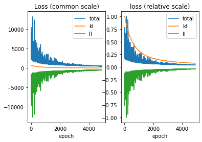
The plot above indicates that the model converged smoothly.
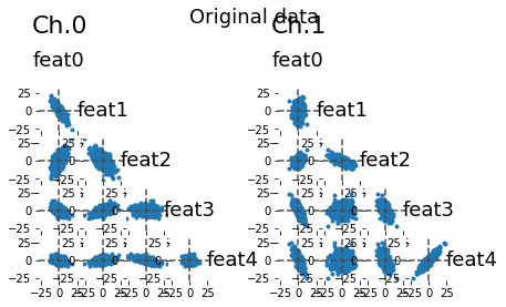
# We can plot the original data, dimension x dimension
lsplom(data, title = 'Original data')
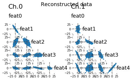
# We can estimate the reconstructed data (decoding from the latent space)
x_hat = model.reconstruct(data)

# Plotting the reconstructed data across dimensions
lsplom(x_hat, title = 'Reconstructed data')
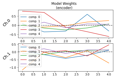
## Plotting the weights of the encoder
plot_weights(model, side = 'encoder')
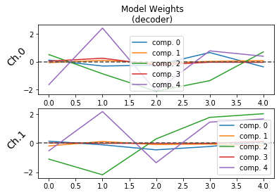
## Plotting the weights of the decoder
plot_weights(model, side = 'decoder')
# Inspecting model parameters

# Decoding parameters
weights_decoding_X = model.vae[0].W_out.weight.data
weights_decoding_Y = model.vae[1].W_out.weight.data

print(weights_decoding_X)
print(weights_decoding_Y)
tensor([[ 0.1148, -0.0684,  0.5098,  0.0365, -1.6451],
        [-0.3095,  0.0943, -0.8667,  0.2497,  2.4173],
        [-0.2510, -0.1134, -2.1274, -0.2352, -2.1068],
        [ 0.6572,  0.0243, -1.3619, -0.0370,  0.7790],
        [-0.3694,  0.0762,  0.7014, -0.0429,  0.3934]])
tensor([[ 0.1395, -0.1859, -1.0957,  0.0222, -0.5188],
        [-0.1095,  0.1167, -2.1759, -0.0054,  2.1793],
        [-0.4565, -0.0929,  0.2947, -0.0118, -1.3441],
        [-0.2269, -0.0548,  1.7775, -0.0096,  1.4515],
        [ 0.1131, -0.1738,  2.0298,  0.1213,  1.6703]])
# Encoding parameters
weights_encoding_X = model.vae[0].W_mu.weight.data
weights_encoding_Y = model.vae[1].W_mu.weight.data

print(weights_encoding_X)
print(weights_encoding_Y)
tensor([[ 0.0909, -0.3644, -0.3227,  0.5998, -0.3149],
        [-0.0150, -0.1016, -0.0240,  0.1764,  0.2570],
        [ 0.0469, -0.1533, -0.2561, -0.1465,  0.0691],
        [ 0.7675,  0.7032, -0.1042, -0.3557, -0.6180],
        [-0.1278,  0.1636, -0.1328,  0.0766,  0.0469]])
tensor([[ 0.1005, -0.1762, -0.4199, -0.2145,  0.1101],
        [-1.1709, -0.0119, -0.3710,  0.0791, -0.7206],
        [-0.1125, -0.1749,  0.0331,  0.1045,  0.1293],
        [ 0.4766, -0.0190,  0.0869, -0.2600,  0.4588],
        [-0.0017,  0.2063, -0.0976,  0.1288,  0.1290]])
# Here we compute the encoding and plot the latent dimensions against our original ground truth for the syntetic data

encoding = model.encode(data)

# Remember: encodings are distributions
print(f'Encoding distribution q for Channel 0: {encoding[0]}')

# with the method "loc" we extract the mean of the distributions
encoding_x = encoding[0].loc.data.numpy()
encoding_y = encoding[1].loc.data.numpy()
Encoding distribution q for Channel 0: Normal(loc: torch.Size([500, 5]), scale: torch.Size([500, 5]))
We note that the estimated encoding is correlated with the original latent dimensions. There seems to be however some redundancy. This motivates the use of a sparse model.
plt.figure(figsize=(12, 12))
for idx,k in enumerate(range(n_components)):

    plt.subplot(n_components,2,2*idx+1)
    plt.scatter(encoding_x[:,k], latents[:,0])
    plt.xlabel(f'mcvae dim {k}')
    plt.ylabel('ground truth 0')

    plt.subplot(n_components,2,2*idx+2)
    plt.scatter(encoding_x[:,k], latents[:,1])
    plt.xlabel(f'mcvae dim {k}')
    plt.ylabel('ground truth 1')

plt.tight_layout()
plt.show()
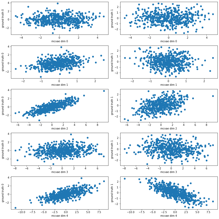
# Initialize sparse mcvae

model_sparse1 = Mcvae(sparse=True, **init_dict)
model_sparse1.to(DEVICE)
print(model_sparse1)
Mcvae(
  (vae): ModuleList(
    (0): VAE(
      (W_out_logvar): Parameter(shape=torch.Size([1, 5]))
      (log_alpha): Parameter(shape=torch.Size([1, 5]))
      (W_mu): Linear(in_features=5, out_features=5, bias=True)
      (W_out): Linear(in_features=5, out_features=5, bias=True)
    )
    (1): VAE(
      (W_out_logvar): Parameter(shape=torch.Size([1, 5]))
      (log_alpha): Parameter(shape=torch.Size([1, 5]))
      (W_mu): Linear(in_features=5, out_features=5, bias=True)
      (W_out): Linear(in_features=5, out_features=5, bias=True)
    )
  )
)
# Optimize
model_sparse1.optimizer = torch.optim.Adam(model_sparse1.parameters(), lr=adam_lr)
load_or_fit(model=model_sparse1, data=data, epochs=n_epochs, ptfile='model_sparse1.pt', force_fit=FORCE_REFIT)
Loading model_sparse1.pt
The sparse model estimates a probability of redundancy associated to each dimension. This means that we can retain only the dimensions with low probability of redundancy. In this case the model correctly identifies only 2 meaningful latent dimensions.
print('Probability of redundancy: ', model_sparse1.dropout.data)
plot_dropout(model_sparse1, sort=False)
Probability of redundancy: tensor([[0.5597, 0.5693, 0.0177, 0.0296, 0.5730]])
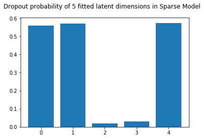
# We fix a redundancy threshold
dropout_threshold = 0.20
# We plot the remaining latent dimensions
keep = (model_sparse1.dropout.squeeze() < dropout_threshold).tolist()
kept_comps = [i for i, kept in enumerate(keep) if kept]
print(f'kept components: {kept_comps}')

plot_latent_space(model_sparse1, data=data, comp=kept_comps);
kept components: [2, 3]
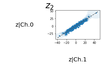
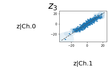
# We repeate the same exercise with the synthetic data with redundant dimensions

data_sparse = [X_ext, Y_ext]
data_sparse = [torch.Tensor(_) for _ in data_sparse]

init_dict = {
    'data': data_sparse,
    'lat_dim': n_components + 3,
}

model_sparse = Mcvae(sparse=True, **init_dict)
model_sparse.to(DEVICE)
print(model_sparse)
Mcvae(
  (vae): ModuleList(
    (0): VAE(
      (W_out_logvar): Parameter(shape=torch.Size([1, 8]))
      (log_alpha): Parameter(shape=torch.Size([1, 8]))
      (W_mu): Linear(in_features=8, out_features=8, bias=True)
      (W_out): Linear(in_features=8, out_features=8, bias=True)
    )
    (1): VAE(
      (W_out_logvar): Parameter(shape=torch.Size([1, 8]))
      (log_alpha): Parameter(shape=torch.Size([1, 8]))
      (W_mu): Linear(in_features=8, out_features=8, bias=True)
      (W_out): Linear(in_features=8, out_features=8, bias=True)
    )
  )
)
# Fit (or load model if existing)
model_sparse.optimizer = torch.optim.Adam(model_sparse.parameters(), lr=adam_lr)
load_or_fit(model=model_sparse, data=data_sparse, epochs=n_epochs, ptfile='model_sparse.pt', force_fit=FORCE_REFIT)
Loading model_sparse.pt
We see that the model recognises again only two meaningful latent dimensions
print('Probability of redundancy: ', model_sparse.dropout.data)
indices = np.where(model_sparse.dropout.data.numpy().flatten() < dropout_threshold)[0]
non_redundant_comps = indices.tolist()
print(f'Non-redundant components: {non_redundant_comps}')
plot_dropout(model_sparse, sort=False)
Probability of redundancy:  tensor([[0.7038, 0.7494, 0.7669, 0.0166, 0.8116, 0.0525, 0.6920, 0.7680]])
Non-redundant components: [3, 5]
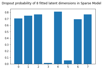
x_hat = model_sparse.reconstruct(data_sparse, dropout_threshold=dropout_threshold)
lsplom(x_hat, title = 'Reconstructed data')
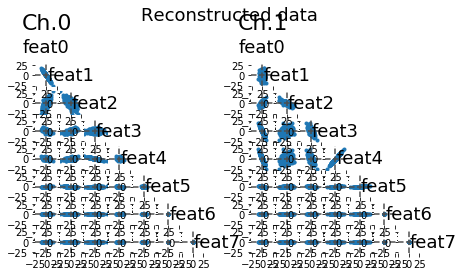
## Plotting the weights of the decoder
plt.figure(figsize=(12, 8))
plot_weights(model_sparse, side = 'decoder')
<Figure size 864x576 with 0 Axes>
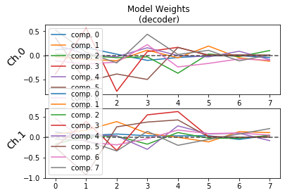
plt.figure(figsize=(12, 8))
plot_weights(model_sparse, side = 'encoder')
<Figure size 864x576 with 0 Axes>
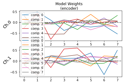
# PLotting estimated encoding vs ground truth

encoding = model_sparse.encode(data_sparse)

encoding_x = encoding[0].loc.detach().numpy()
encoding_y = encoding[1].loc.detach().numpy()

plt.figure(figsize=(12, 12))
for idx,k in enumerate(indices):
  plt.subplot(len(indices),2,2*idx+1)
  plt.scatter(encoding_x[:,k], latents[:,0])
  plt.xlabel(str('mcvae dim ') + str(k))
  plt.ylabel('ground truth 0')
  plt.subplot(len(indices),2,2*idx+2)
  plt.scatter(encoding_x[:,k], latents[:,1])
  plt.xlabel(str('mcvae dim ') + str(k))
  plt.ylabel('ground truth 1')

plt.show()
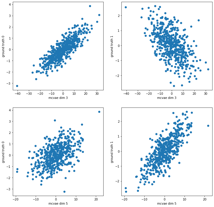
plot_latent_space(model_sparse, data_sparse, comp=non_redundant_comps);
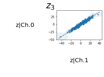
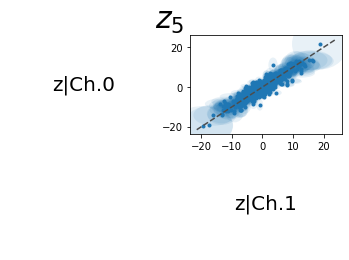
Increasing the number of channels
In this section we explore the use of the model on data with multiple modalities (or channels)
# generating a new modality Z
# This modality has meaningful as well as redundant dimensions

size_z = 10

size_z_redundant = 4

np.random.seed(37)
Z_redundant = np.random.randn(n, size_z_redundant)  # pure noise

transform_z = np.random.randint(-8, 8, size=(2, size_z))

Z = latents.dot(transform_z) + 2*np.random.normal(size=(n, size_z))
Z = np.hstack([Z, Z_redundant])

print(X_ext.shape,Y_ext.shape, Z.shape)
(500, 8) (500, 8) (500, 14)
# Initialize the model
data_multi = [X_ext, Y_ext, Z]
data_multi = [torch.Tensor(_) for _ in data_multi]

init_dict = {
    'data': data_multi, # [X, Y, Z]
    'lat_dim': n_components + 3,
}

model_multi = Mcvae(sparse=True, **init_dict)
model_multi.to(DEVICE)
print(model_multi)
Mcvae(
  (vae): ModuleList(
    (0): VAE(
      (W_out_logvar): Parameter(shape=torch.Size([1, 8]))
      (log_alpha): Parameter(shape=torch.Size([1, 8]))
      (W_mu): Linear(in_features=8, out_features=8, bias=True)
      (W_out): Linear(in_features=8, out_features=8, bias=True)
    )
    (1): VAE(
      (W_out_logvar): Parameter(shape=torch.Size([1, 8]))
      (log_alpha): Parameter(shape=torch.Size([1, 8]))
      (W_mu): Linear(in_features=8, out_features=8, bias=True)
      (W_out): Linear(in_features=8, out_features=8, bias=True)
    )
    (2): VAE(
      (W_out_logvar): Parameter(shape=torch.Size([1, 14]))
      (log_alpha): Parameter(shape=torch.Size([1, 8]))
      (W_mu): Linear(in_features=14, out_features=8, bias=True)
      (W_out): Linear(in_features=8, out_features=14, bias=True)
    )
  )
)
# Fit (or load)
model_multi.optimizer = torch.optim.Adam(model_multi.parameters(), lr=adam_lr)
load_or_fit(model=model_multi, data=data_multi, epochs=n_epochs, ptfile='model_multi.pt', force_fit=FORCE_REFIT)
Loading model_multi.pt
print('Probability of redundancy: ', model_multi.dropout.data.numpy())
indices = np.where(model_multi.dropout.data.numpy().flatten() < dropout_threshold)[0]
print('Non-redundant components: ', indices)
plot_dropout(model_multi, sort=False)

encoding = model_multi.encode(data_multi)

encoding_x = encoding[0].loc.detach().numpy()
encoding_y = encoding[1].loc.detach().numpy()
encoding_z = encoding[2].loc.detach().numpy()

plt.figure(figsize=(12, 12))
for idx,k in enumerate(indices):
    plt.subplot(len(indices),2,2*idx+1)
    plt.scatter(encoding_z[:,k], latents[:,0])
    plt.xlabel(str('mcvae dim ') + str(k))
    plt.ylabel('ground truth 0')
    plt.subplot(len(indices),2,2*idx+2)
    plt.scatter(encoding_z[:,k], latents[:,1])
    plt.xlabel(str('mcvae dim ') + str(k))
    plt.ylabel('ground truth 1')

plt.show()
Probability of redundancy:  [[0.03285351 0.39449245 0.00762853 0.60119134 0.59263474 0.6564989
  0.25333416 0.3858575 ]]
Non-redundant components:  [0 2]
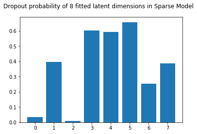
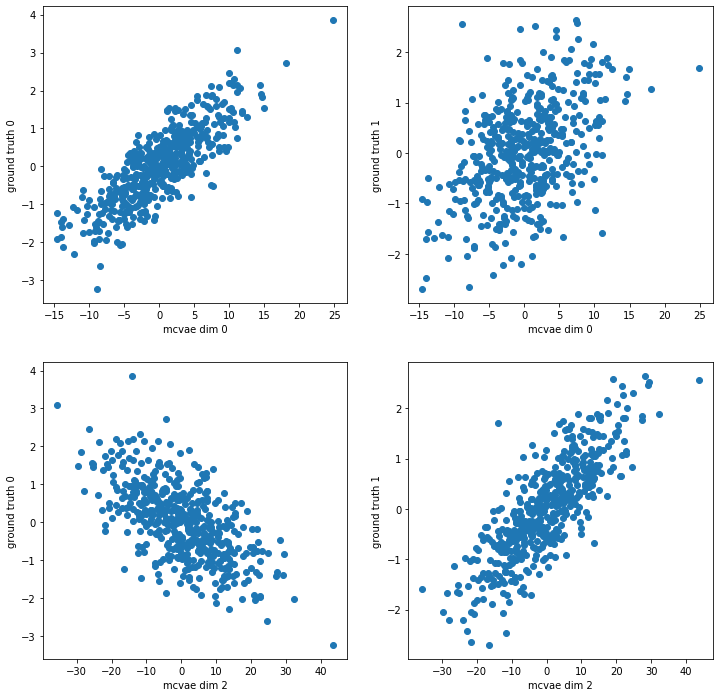
The multi-channel variational autoencoder allows to predict each channel from any other.
# We compute the reconstruction of the data from the encoding
z = [_.sample() for _ in encoding]  # sample the encoding distributions
p = model_multi.decode(z)  # compute the decoding distributions

# This variable has several dimensions over two indices:
# the first index indicates the modality to decode(0:x, 1:y, 3:z, ...)
# the second index indicates the modality from which the encoding is done (0:x, 1:y, 3:z, ...)

# p[x][z]: p(x|z)
decoding_x_from_x = p[0][0].loc.data.numpy()
decoding_x_from_y = p[0][1].loc.data.numpy()
decoding_x_from_z = p[0][2].loc.data.numpy()
plt.figure(figsize=(18, 10))
plt.subplot(2,3,1)
plt.scatter(X_ext[:,0], decoding_x_from_x[:,0])
plt.title('decoding X from X')
plt.xlabel('X0')
plt.ylabel('X0 from latent X')
plt.subplot(2,3,2)
plt.scatter(X_ext[:,0], decoding_x_from_y[:,0])
plt.title('decoding X from Y')
plt.ylabel('X0 from latent Y')
plt.xlabel('X0')
plt.subplot(2,3,3)
plt.scatter(X_ext[:,0], decoding_x_from_z[:,0])
plt.title('decoding X from Z')
plt.xlabel('X0')
plt.ylabel('X0 from latent Z')
plt.subplot(2,3,4)
plt.scatter(decoding_x_from_x[:,0], decoding_x_from_y[:,0])
plt.title('decoding X vs decoding Y')
plt.xlabel('X0 from latent X')
plt.ylabel('X0 from latent Y')
plt.subplot(2,3,5)
plt.scatter(decoding_x_from_x[:,0], decoding_x_from_z[:,0])
plt.title('decoding Y vs decoding Z')
plt.xlabel('X0 from latent X')
plt.ylabel('X0 from latent Z')
plt.subplot(2,3,6)
plt.scatter(decoding_x_from_y[:,0], decoding_x_from_z[:,0])
plt.title('decoding Y vs decoding Z')
plt.xlabel('X0 from latent Y')
plt.ylabel('X0 from latent Z')
plt.tight_layout()
plt.show()
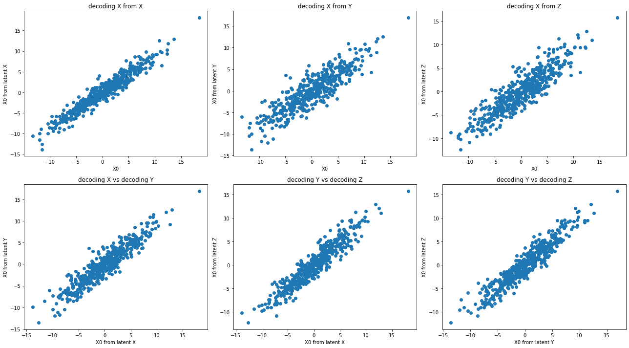
Application to (pseudo-) neurological data
We are going to load volumetric and cognitive data for a synthetic sample generated from the ADNI dataset. The exercise consists in applying the methods seen so far to understand the relationship between this kind of variables.
import pandas as pd

adni = pd.read_csv('https://marcolorenzi.github.io/material/pseudo_adni.csv')

brain_volume_cols = ['WholeBrain.bl', 'Ventricles.bl', 'Hippocampus.bl', 'MidTemp.bl', 'Entorhinal.bl']
cognition_cols = ['CDRSB.bl', 'ADAS11.bl', 'MMSE.bl', 'RAVLT.immediate.bl', 'RAVLT.learning.bl', 'RAVLT.forgetting.bl', 'FAQ.bl']

adni[brain_volume_cols]
| WholeBrain.bl | Ventricles.bl | Hippocampus.bl | MidTemp.bl | Entorhinal.bl | |
|---|---|---|---|---|---|
| 0 | 0.684331 | 0.012699 | 0.003786 | 0.012678 | 0.002214 |
| 1 | 0.735892 | 0.012803 | 0.004866 | 0.015071 | 0.003041 |
| 2 | 0.738731 | 0.030492 | 0.004300 | 0.012419 | 0.002316 |
| 3 | 0.696179 | 0.032797 | 0.004720 | 0.012312 | 0.002593 |
| 4 | 0.841806 | 0.004030 | 0.006820 | 0.016948 | 0.002896 |
| ... | ... | ... | ... | ... | ... |
| 995 | 0.767153 | 0.011417 | 0.005209 | 0.012879 | 0.002208 |
| 996 | 0.695168 | 0.011908 | 0.004641 | 0.012534 | 0.002197 |
| 997 | 0.628691 | 0.041537 | 0.003478 | 0.010870 | 0.001939 |
| 998 | 0.714763 | 0.020461 | 0.004713 | 0.013989 | 0.001981 |
| 999 | 0.691858 | 0.030349 | 0.004237 | 0.011439 | 0.002419 |
1000 rows × 5 columns
volumes_value = adni[brain_volume_cols].values

# Standardization of volumetric measures
volumes_value = (volumes_value - volumes_value.mean(0)) / volumes_value.std(0)
adni[cognition_cols]
| CDRSB.bl | ADAS11.bl | MMSE.bl | RAVLT.immediate.bl | RAVLT.learning.bl | RAVLT.forgetting.bl | FAQ.bl | |
|---|---|---|---|---|---|---|---|
| 0 | 1 | 8 | 27.0 | 23.739439 | 4.0 | 5.821573 | 3 |
| 1 | 0 | 0 | 30.0 | 64.933800 | 9.0 | 4.001653 | 0 |
| 2 | 0 | 8 | 24.0 | 36.987722 | 3.0 | 6.876316 | 0 |
| 3 | 0 | 3 | 29.0 | 50.314425 | 5.0 | 4.733481 | 3 |
| 4 | 0 | 0 | 30.0 | 57.217830 | 9.0 | 7.225401 | 0 |
| ... | ... | ... | ... | ... | ... | ... | ... |
| 995 | 1 | 2 | 29.0 | 61.896022 | 8.0 | 1.663102 | 0 |
| 996 | 0 | 1 | 29.0 | 62.083170 | 8.0 | 5.241477 | 1 |
| 997 | 3 | 14 | 24.0 | 22.289059 | 2.0 | 5.437600 | 7 |
| 998 | 0 | 13 | 26.0 | 31.650504 | 2.0 | 1.669603 | 4 |
| 999 | 0 | 15 | 28.0 | 29.089863 | 3.0 | 7.703384 | 4 |
1000 rows × 7 columns
cognition_value = adni[cognition_cols].values

# Standardization of cognitive measures
cognition_value = (cognition_value - cognition_value.mean(0)) / cognition_value.std(0)
Exercise (a). Use PLS to model the relationship between cognitive variables and brain volumes. How many latent components are needed?
Exercise (b). Explore the PLS model weights to interpret the relationship between the variables identified by the model.
McVAE
In this last application we apply the multichannel autoencoder to the pseudo-ADNI data, for jointly modeling different modalities across individuals. We focus on the joint analysis of:
brain volumes;
sociodemographic information (e.g. age, sex, scholarity);
cognition;
apoe genotype;
fluid biomarkers (abeta and tay concentrations in the CSF).
We first import and standardize the different data modalities.
adni = pd.read_csv('https://marcolorenzi.github.io/material/pseudo_adni.csv')

normalize = lambda _: (_ - _.mean(0))/_.std(0)

volume_cols = ['WholeBrain.bl', 'Ventricles.bl', 'Hippocampus.bl', 'MidTemp.bl', 'Entorhinal.bl']
volumes_value = adni[volume_cols].values
volumes_value = normalize(volumes_value)

demog_cols = ['SEX', 'AGE', 'PTEDUCAT']
demog_value = adni[demog_cols].values
demog_value = normalize(demog_value)

cognition_cols = ['CDRSB.bl', 'ADAS11.bl', 'MMSE.bl', 'RAVLT.immediate.bl', 'RAVLT.learning.bl', 'RAVLT.forgetting.bl', 'FAQ.bl']
cognition_value = adni[cognition_cols].values
cognition_value = normalize(cognition_value)

apoe_cols = ['APOE4']
apoe_value = adni[apoe_cols].values
apoe_value = normalize(apoe_value)

fluid_cols = ['ABETA.MEDIAN.bl', 'PTAU.MEDIAN.bl', 'TAU.MEDIAN.bl']
fluid_value = adni[fluid_cols].values
fluid_value = normalize(fluid_value)

# Creating a list with multimodal data
data_adni = [volumes_value, demog_value, cognition_value, apoe_value, fluid_value]
adni_cols = [volume_cols, demog_cols, cognition_cols, apoe_cols, fluid_cols]

# Transform as a pytorch Tensor for compatibility
data_adni = [torch.Tensor(_) for _ in data_adni]

print(f'We have {len(data_adni)} channels in total as an input for the model')
We have 5 channels in total as an input for the model
##############################################
## FIT a Sparse Mcvae with Pseudo-Adni data ##
##############################################

# create an instance of the model

model_adni = Mcvae(data = data_adni, lat_dim = 5, sparse=True)
model_adni.to(DEVICE)
print(model_adni)

# set up the optimizer

adam_lr = 1e-2
n_epochs = 6000

model_adni.optimizer = torch.optim.Adam(model_adni.parameters(), lr=1e-2)

# fit
load_or_fit(model=model_adni, data=data_adni, epochs=6000, ptfile='model_adni.pt', force_fit=FORCE_REFIT)
Mcvae(
  (vae): ModuleList(
    (0): VAE(
      (W_out_logvar): Parameter(shape=torch.Size([1, 5]))
      (log_alpha): Parameter(shape=torch.Size([1, 5]))
      (W_mu): Linear(in_features=5, out_features=5, bias=True)
      (W_out): Linear(in_features=5, out_features=5, bias=True)
    )
    (1): VAE(
      (W_out_logvar): Parameter(shape=torch.Size([1, 3]))
      (log_alpha): Parameter(shape=torch.Size([1, 5]))
      (W_mu): Linear(in_features=3, out_features=5, bias=True)
      (W_out): Linear(in_features=5, out_features=3, bias=True)
    )
    (2): VAE(
      (W_out_logvar): Parameter(shape=torch.Size([1, 7]))
      (log_alpha): Parameter(shape=torch.Size([1, 5]))
      (W_mu): Linear(in_features=7, out_features=5, bias=True)
      (W_out): Linear(in_features=5, out_features=7, bias=True)
    )
    (3): VAE(
      (W_out_logvar): Parameter(shape=torch.Size([1, 1]))
      (log_alpha): Parameter(shape=torch.Size([1, 5]))
      (W_mu): Linear(in_features=1, out_features=5, bias=True)
      (W_out): Linear(in_features=5, out_features=1, bias=True)
    )
    (4): VAE(
      (W_out_logvar): Parameter(shape=torch.Size([1, 3]))
      (log_alpha): Parameter(shape=torch.Size([1, 5]))
      (W_mu): Linear(in_features=3, out_features=5, bias=True)
      (W_out): Linear(in_features=5, out_features=3, bias=True)
    )
  )
)
Loading model_adni.pt
# Check convergence
plot_loss(model_adni)
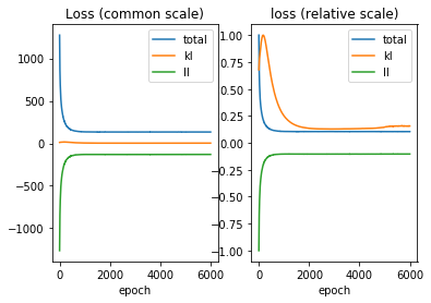
The model identified only a significant dimension, that we are going to store and analyze:
# Identify the most significant latent dimension
plot_dropout(model_adni)
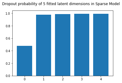
kept_dim = 0
The weights give us a nice way to interpret how the different modalities interact together.
# Plot the decoding weights (the generative parameters)
# associated to the non-redundant dimension latent dimension

# Store the weights (use the practical "dot" notation model.vae[i].W_out.weight)
decoding_weights = [vae.W_out.weight.data[:, kept_dim] for vae in model_adni]

# Plot
plt.figure(figsize=(12, 12))
for i in range(len(data_adni)):
    plt.subplot(5,1,i+1)
    plt.bar(np.arange(len(decoding_weights[i])), decoding_weights[i], tick_label = adni_cols[i])
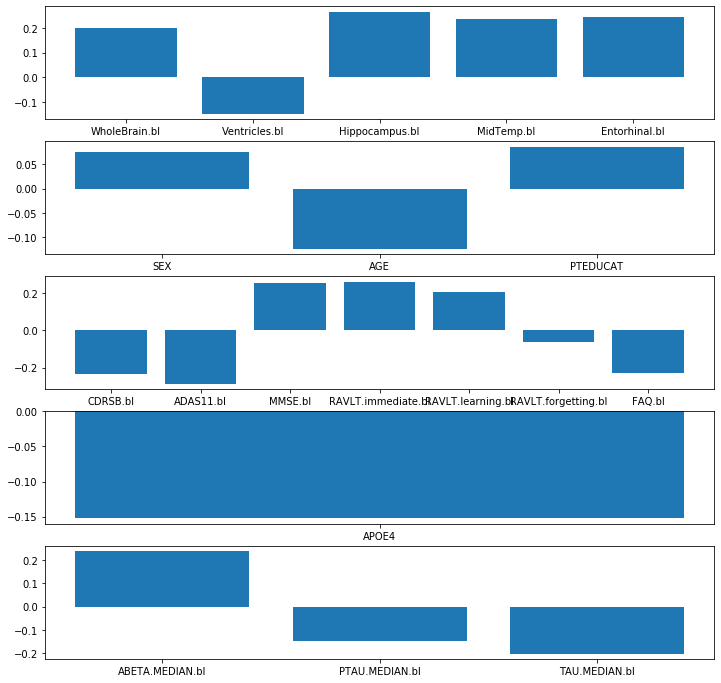
Once the model is learnt we can use it for prediction. For example we can predict brain volumes from the cognitive data:
# Predict volumes (channel 0) from cognition (channel 2)

# Solution 1

# Encode everything
q = model_adni.encode(data_adni)
# Take the mean of every encoded distribution q
z = [qi.loc for qi in q]
# Decode all
p = model_adni.decode(z)
# Extract what you need: p(x|z) or p[x][z] or p[decoder output channel][encoder input chanenl]
decoding_volume_from_cognition = p[0][2].loc.data.numpy()

# Solution 2

# Encode the cognition (ch 2)
q2 = model_adni.vae[2].encode(data_adni[2])
# Take the mean of q (location in pytorch jargon)
z2 = q2.loc
# Decode through the brain volumes decoder (ch 0)
p0 = model_adni.vae[0].decode(z2)
# Take the mean
decoding_volume_from_cognition = p0.loc.data.numpy()
# Plot the predicted volumes against the true ones.
# Create one plot per volumetric feature

plt.figure(figsize=(12, 28))

for i in range(len(volume_cols)):
    plt.subplot(5,1,i+1)
    plt.scatter(decoding_volume_from_cognition[:,i], volumes_value[:,i])
    plt.title('reconstruction ' + volume_cols[i])
    plt.xlabel('predicted')
    plt.ylabel('target')
plt.show()
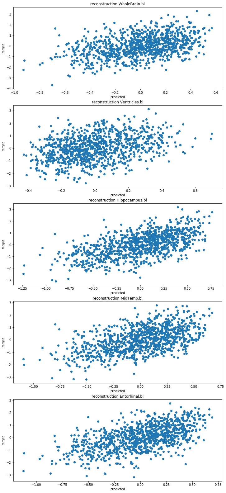
We are finally going to compare the multichannel model with the standard PLS modeling cognition and brain volumes jointly:
# FIT a PLS model to predict: cognition -> volume

plsca = PLSCanonical(n_components=1, scale = False)
plsca.fit(cognition_value, volumes_value)
PLSCanonical(n_components=1, scale=False)
# Compare (plot) the prediction of PLS against the true values and against the predictions of Mcvae.
# Are they correlated?

predicted_plsca = plsca.predict(cognition_value)

plt.figure(figsize=(26, 18))

for i in range(5):
    plt.subplot(10,2,2*i+1)
    plt.scatter(predicted_plsca[:,i], volumes_value[:,i])
    plt.title('reconstruction' + volume_cols[i])
    plt.xlabel('predicted')
    plt.ylabel('target')

for i in range(5):
    plt.subplot(10,2,2*i+2)
    plt.scatter(predicted_plsca[:,i], decoding_volume_from_cognition[:,i])
    plt.title('reconstruction' + volume_cols[i])
    plt.xlabel('cca')
    plt.ylabel('mcvae')

plt.show()
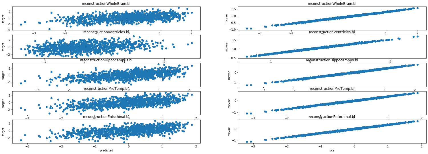
# Compare average reconstruction errors between PLS and Mcvae
print('Reconstruction error:')
print(f'PLS: {((predicted_plsca-volumes_value)**2).sum()}')
print(f'mcvae: {((decoding_volume_from_cognition-volumes_value)**2).sum()}')
Reconstruction error:
PLS: 4631.245631476227
mcvae: 3964.8306431191213